Amazing Algorithms

For Solving Problems in Software


Barry S. Stahl

Principal Engineer - AZNerds.net

@bsstahl@cognitiveinheritance.com

https://CognitiveInheritance.com

Transparent Half Width Image 800x800.png

Favorite Physicists & Mathematicians

Favorite Physicists

  1. Harold "Hal" Stahl
  2. Carl Sagan
  3. Richard Feynman
  4. Marie Curie
  5. Nikola Tesla
  6. Albert Einstein
  7. Neil deGrasse Tyson
  8. Niels Bohr
  9. Galileo Galilei
  10. Michael Faraday

Other notables: Stephen Hawking, Edwin Hubble, Leonard Susskind, Christiaan Huygens

Favorite Mathematicians

  1. Ada Lovelace
  2. Alan Turing
  3. Tim Berners-Lee
  4. Isaac Newton
  5. Emmy Noether
  6. Johannes Kepler
  7. René Descartes
  8. George Boole
  9. Carl Friedrich Gauss
  10. Grace Hopper

Other notables: Blaise Pascal, Daphne Koller, Grady Booch, Evelyn Berezin, Pascal Van Hentenryck

Fediverse Supporter

Logos.png

Some OSS Projects I Run

  1. Liquid Victor : Media tracking and aggregation [used to assemble this presentation]
  2. Prehensile Pony-Tail : A static site generator built in c#
  3. TestHelperExtensions : A set of extension methods helpful when building unit tests
  4. Conference Scheduler : A conference schedule optimizer
  5. IntentBot : A microservices framework for creating conversational bots on top of Bot Framework
  6. LiquidNun : Library of abstractions and implementations for loosely-coupled applications
  7. Toastmasters Agenda : A c# library and website for generating agenda's for Toastmasters meetings
  8. ProtoBuf Data Mapper : A c# library for mapping and transforming ProtoBuf messages

http://GiveCamp.org

GiveCamp.png

Achievement Unlocked

bss-100-achievement-unlocked-1024x250.png

Agenda

  • 08:45 - 09:00 : Intro and Modeling

  • 09:00 - 10:30 : Dynamic Programming

  • 10:30 - 11:00 : Break

  • 11:00 - 11:15 : Genetic Algorithms

  • 11:15 - 12:15 : Classification & Clustering

  • 12:15 - 1:15 : Lunch

  • 1:15 - 2:45 : Simplex Algorithm (CP, LP & MIP)

  • 2:45 - 3:15 : Break

  • 3:15 - 3:45 : Best-Path Algorithms

  • 3:45 - 4:15 : Cost-Minimization Algorithms

  • 4:15 - 4:30 : Training Neural Networks

  • 4:30 - 4:45 : Q&A and Wrap-up

AI Simulates A Rational Actor

Attempts to make the best possible decision​ based on the model and the data

  • Model - Our description of the problem
  • Data - Our understanding of the state of the domain
A Rational Actor 800x800.jpeg

Models are the Blueprint

The success of a problem-solving algorithm is often determined before the algorithm even runs -- by how the problem is modeled

Models are the Blueprint 800x800.jpg

Modeling

  • Modeling defines the problem space
    • What’s included & what’s ignored
    • Poor models lead to irrelevant solutions
  • Modeling shapes the solution strategy
    • Logical models » OOP or Rules Engines
    • Graph models » traversal algorithms
    • Constraint models » LP or MIP
    • Probabilistic models » Neural/Bayesian Networks
  • Modeling can determine tractability
    • Some formulations make problems NP-hard
    • Others reveal polynomial-time solutions
    • Examples
      • Conference Scheduling with LP vs MIP
      • Traveling Salesman with OOP

Workshop Goals

  • Describe these algorithms
    • Show models that work well with each type of problem
    • Describe sample implementations for your use
    • Provide intuition as to why they work as they do
Models and Algorithms 800x800.jpg

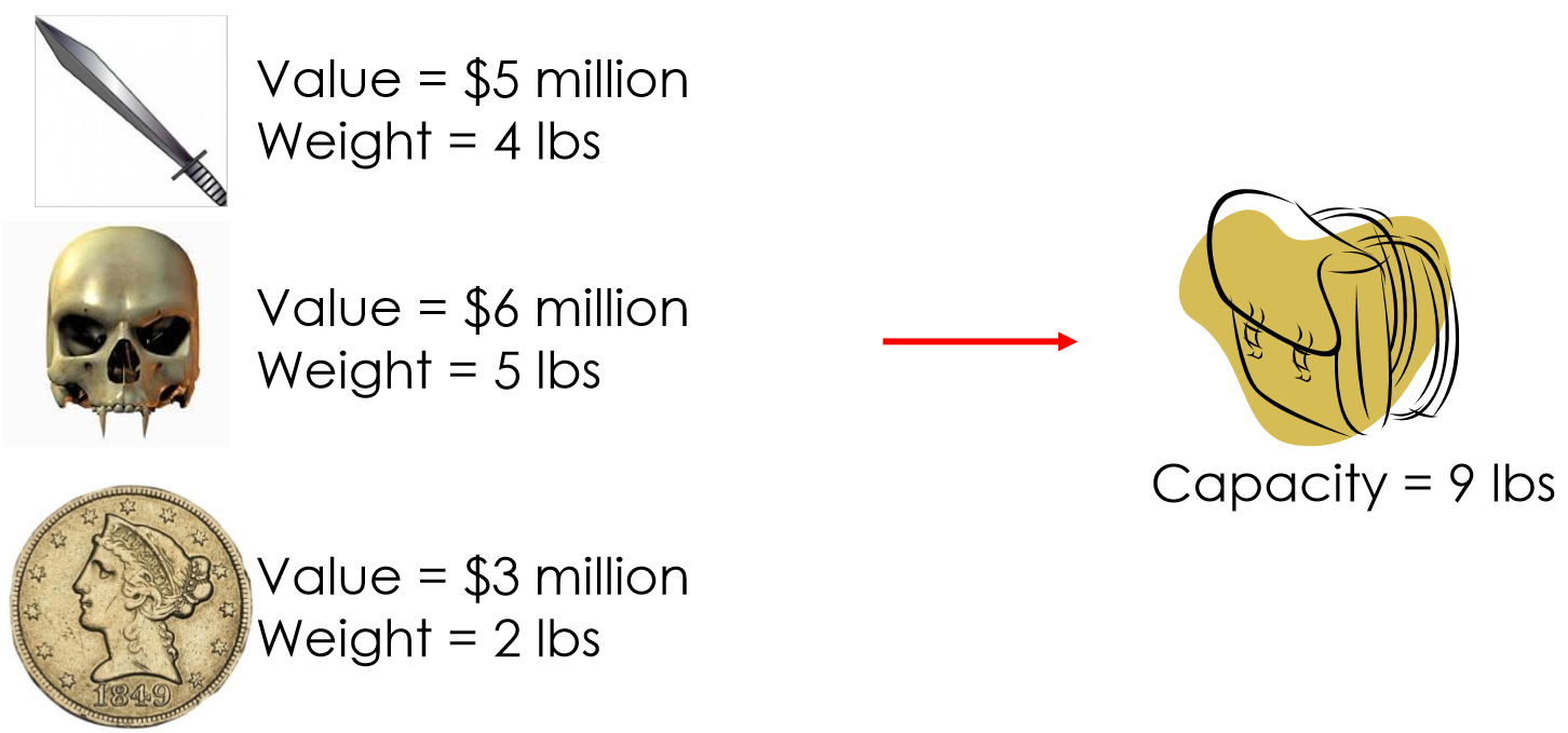
Knapsack Problems

  • A family of combinatorial optimization problems
  • Goal
    • Select a subset of items from a larger set
    • Without exceeding resource constraints
    • Such that total value is maximized
Knapsack 800x800.jpeg

Memoization

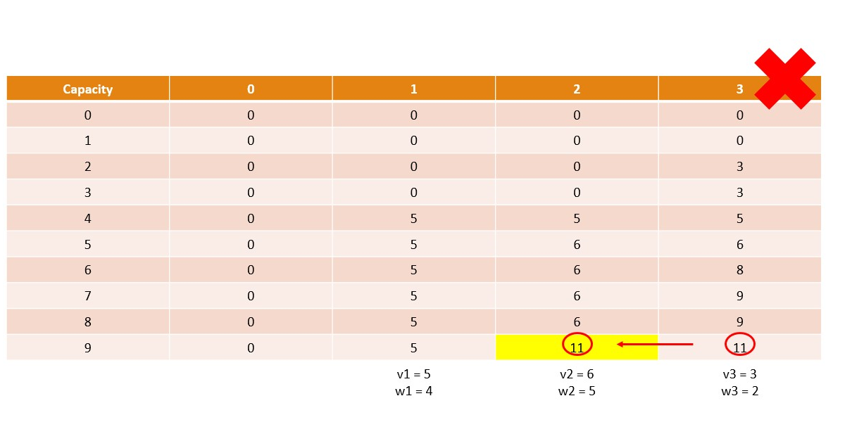
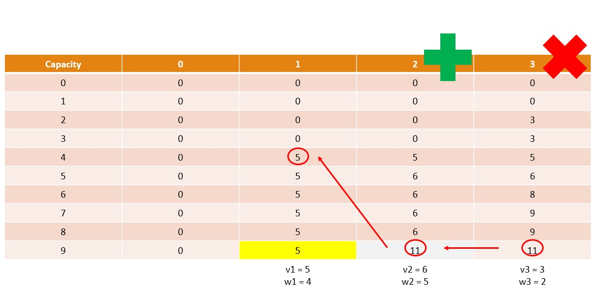
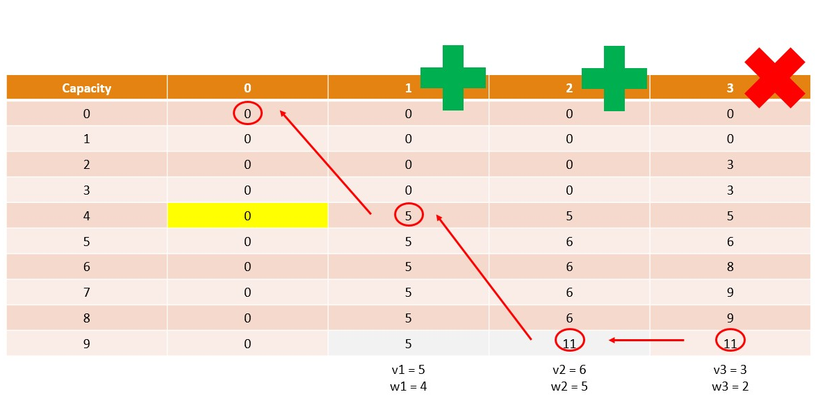
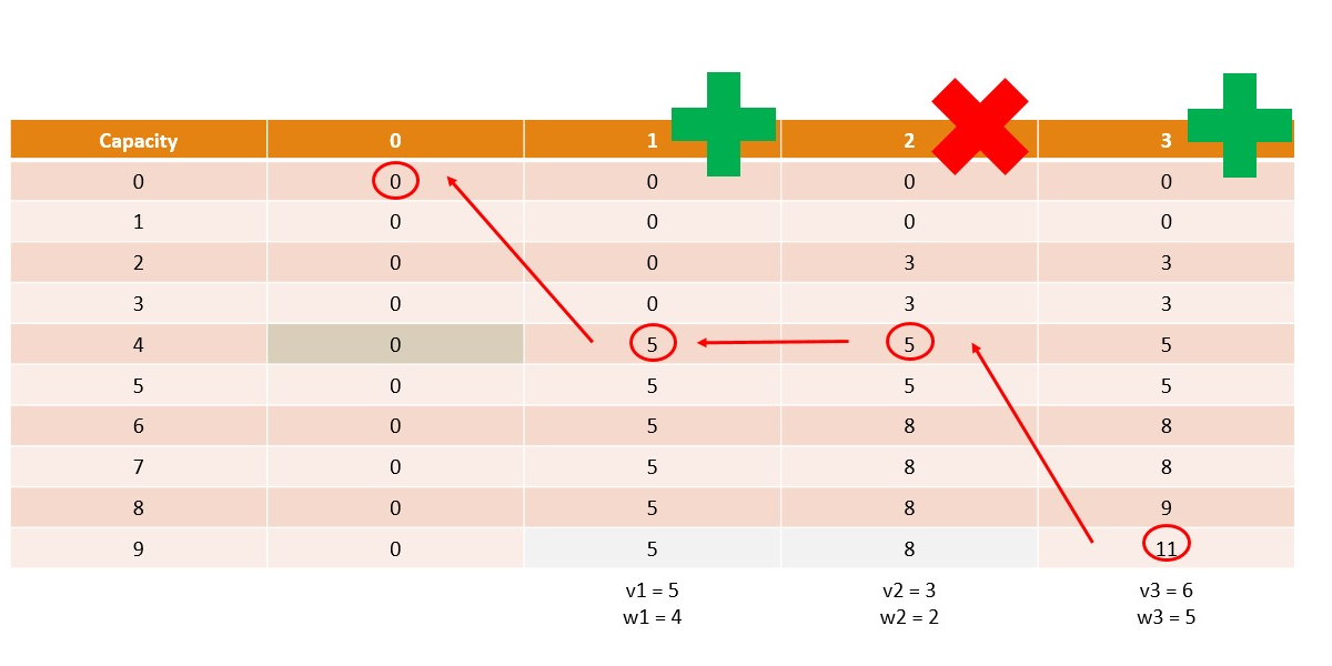
Store the results of function calls for reuse when the same inputs occur again

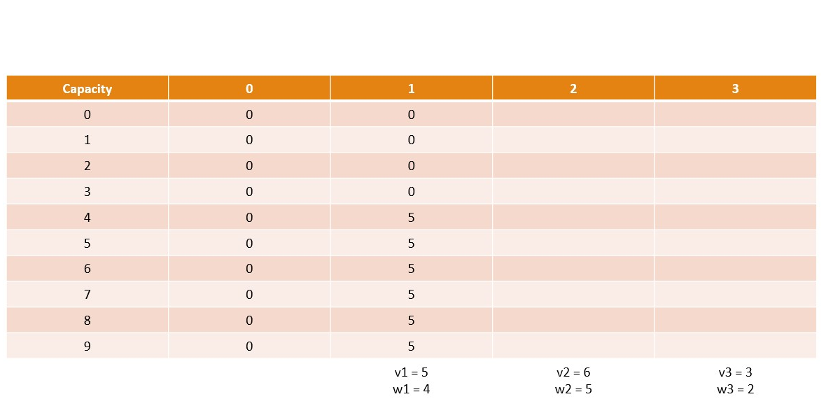
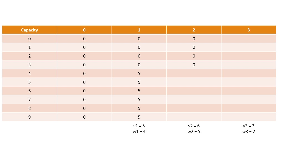
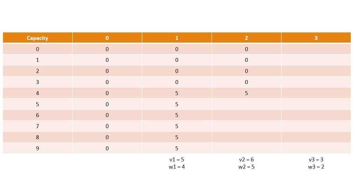
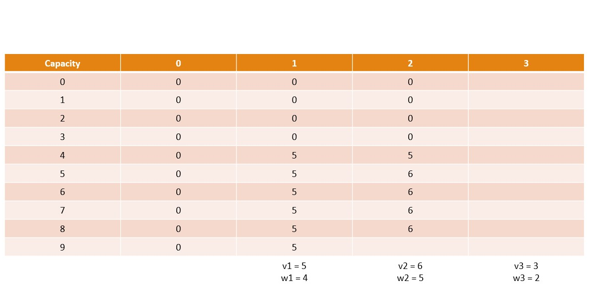
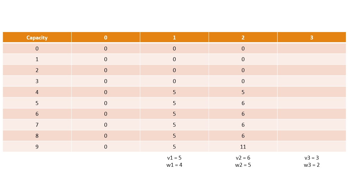
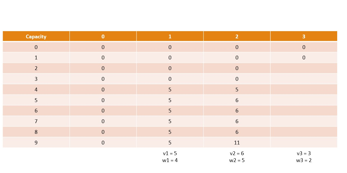
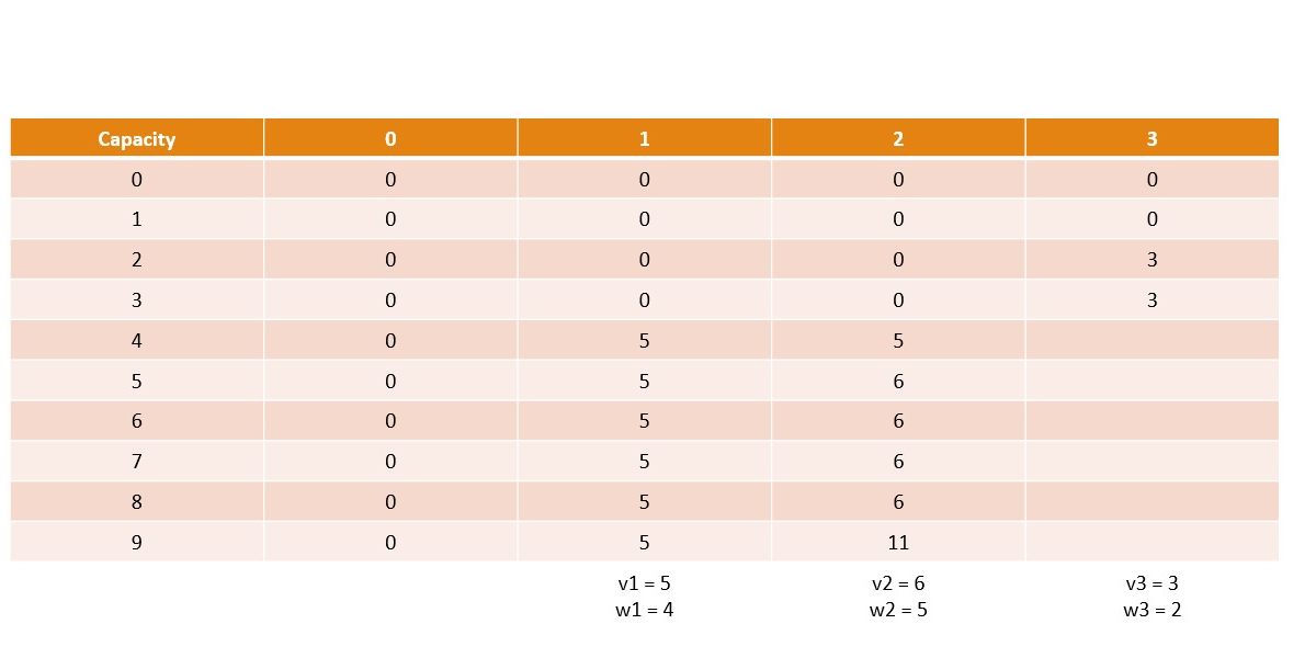
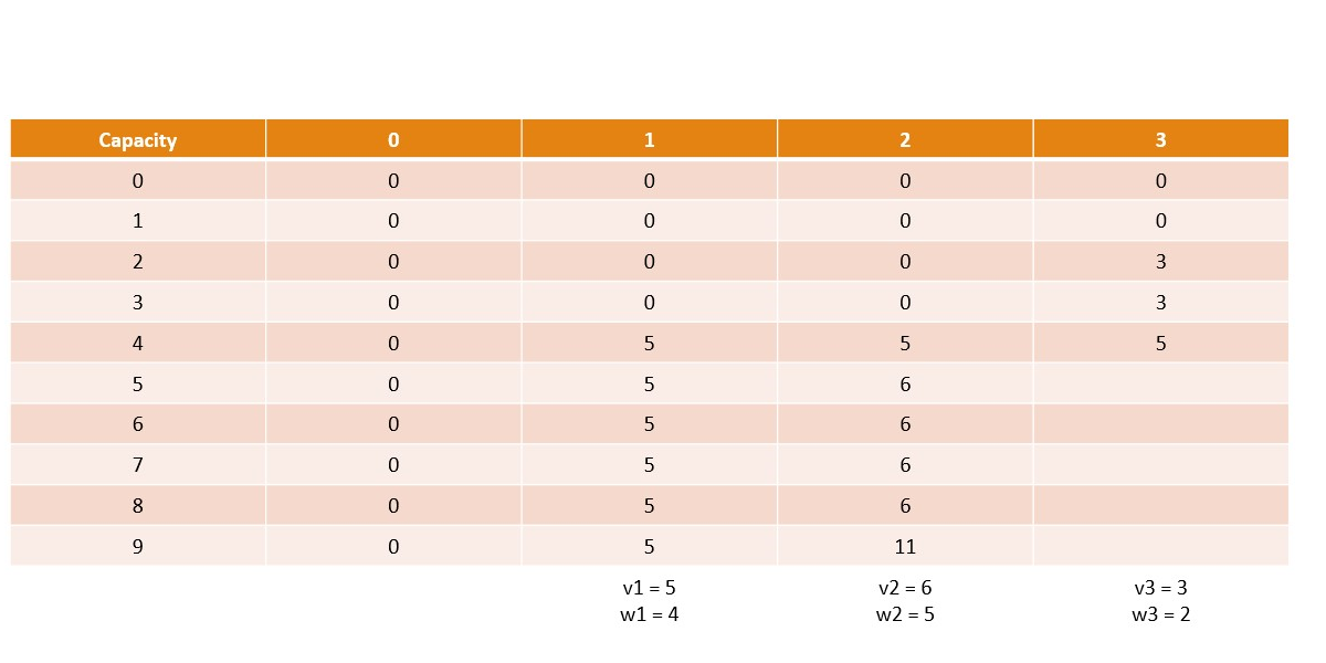
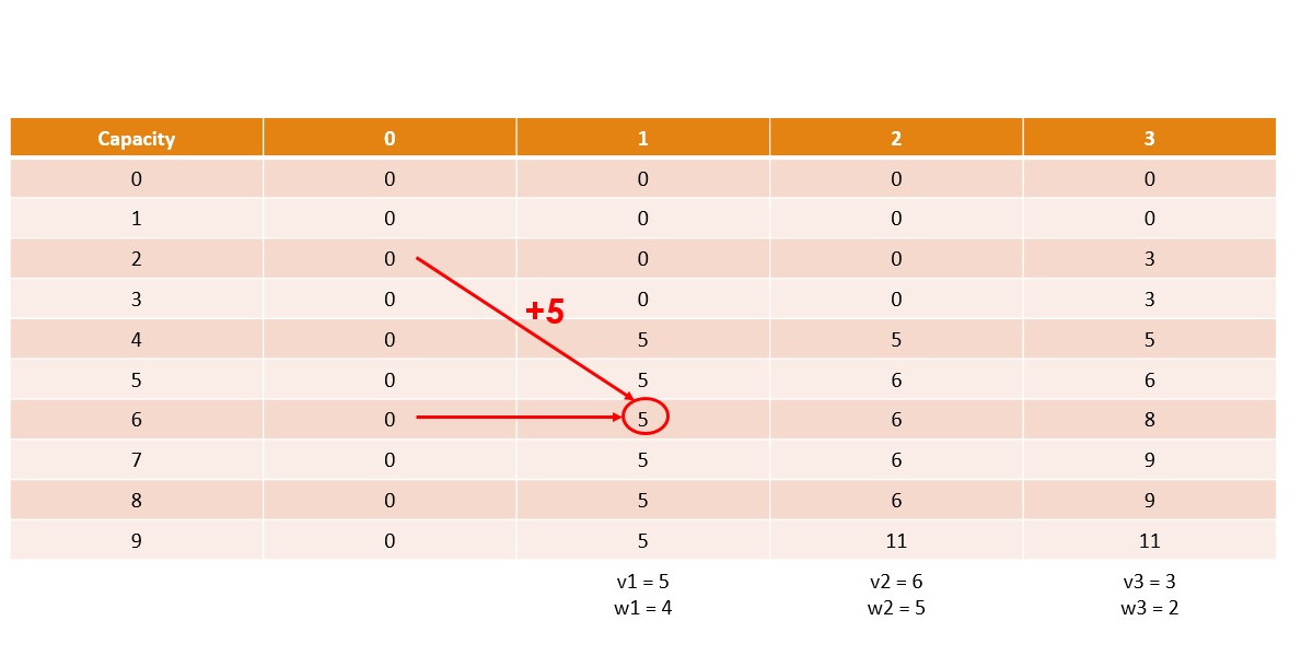
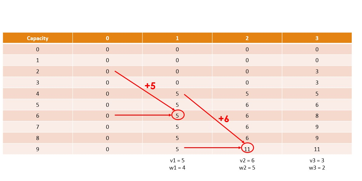
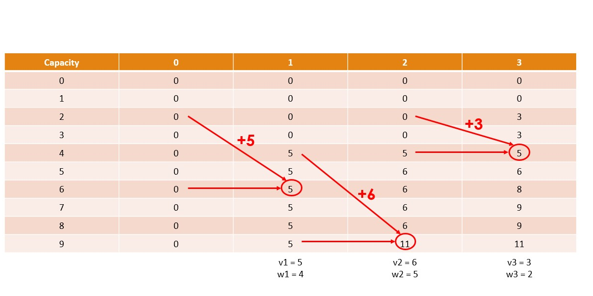
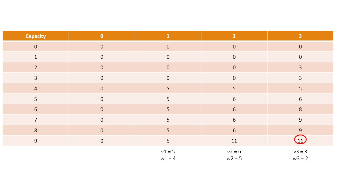
  • Goal: Compute the nth Fibonacci number
    • F(n) = F(n-1) + F(n-2)
  • Naïve Recursion
    • Recomputes each subproblem multiple times
    • O(2n) Problem - Exponential time
  • With Memoization
    • Store results of F(k)
    • Reuse stored values
    • O(n) Problem - Linear Time
Memoization 800x800.jpeg

Decision Variables

In optimization, decision variables are the values we are solving for

  • In knapsack problems, each candidate item has a boolean decision variable

    • \(x_i = 1\) means include item \(i\)
    • \(x_i = 0\) means exclude item \(i\)
  • The goal is to choose the combination of \(x_1, x_2, ... x_n\) that gives the best valid knapsack

DecisionVars-800x800.png

Canonical Knapsack Problem

Knapsack Problem.png

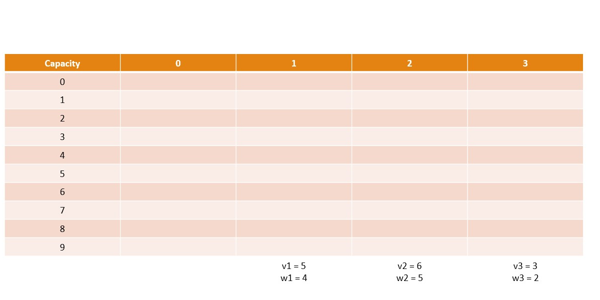
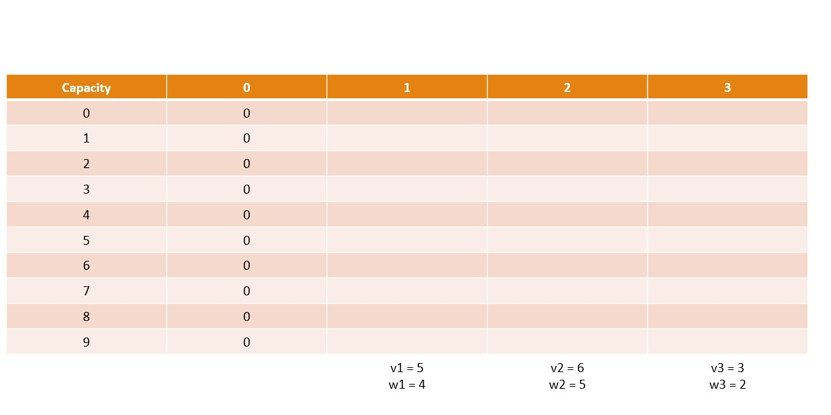
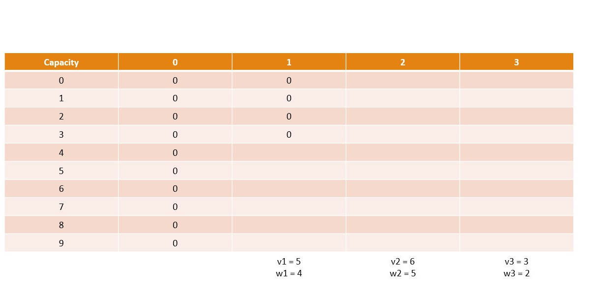
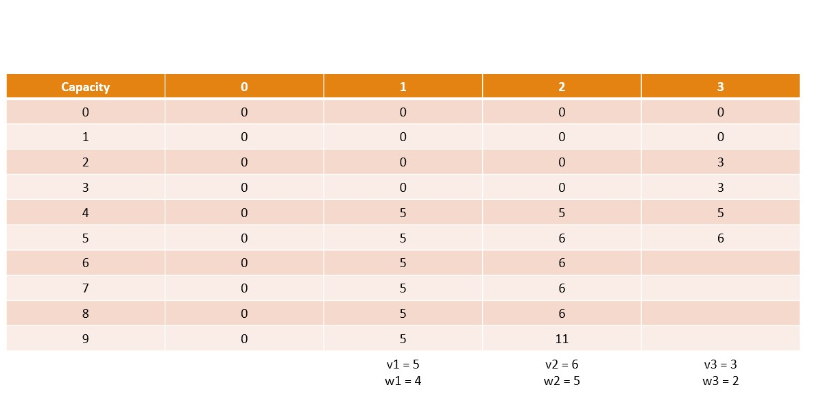
Memoization

Slide7_1200x600.jpg

Memoization

Slide8_1200x600.jpg

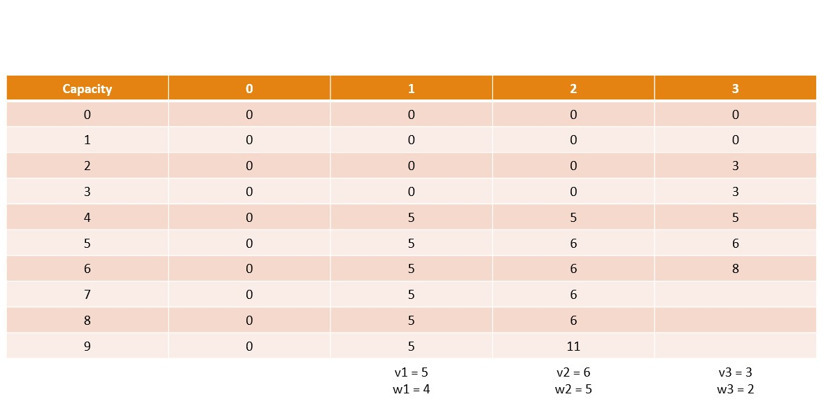
Memoization

Slide9_1200x600.jpg

Memoization

Slide10_1200x600.jpg

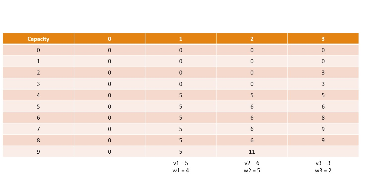
Memoization

Slide11_1200x600.jpg

Memoization

Slide12_1200x600.jpg

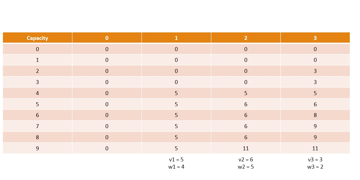
Memoization

Slide13_1200x600.jpg

Memoization

Slide14_1200x600.jpg

Memoization

Slide15_1200x600.jpg

Memoization

Slide16_1200x600.jpg

Memoization

Slide17_1200x600.jpg

Memoization

Slide18_1200x600.jpg

Memoization

Slide19_1200x600.jpg

Memoization

Slide20_1200x600.jpg

Memoization

Slide21_1200x600.jpg

Memoization

Slide22_1200x600.jpg

Memoization

Slide23_1200x600.jpg

Memoization

Slide24_1200x600.jpg

Memoization

Slide25_1200x600.jpg

Memoization

Slide26_1200x600.jpg

Memoization

Slide27_1200x600.jpg

Memoization

Slide28_1200x600.jpg

Memoization

Slide29_1200x600.jpg

Dynamic Programming

A mathematical optimization technique

  • Best for solving problems that can be described recursively
  • Breaks the problem into smaller sub-problems​
  • Solves each small problem only once​
  • Guarantees an optimal solution​

Combinatorial Explosion

Items ($n$) DP calculations Brute-force calculations
3 27 8
30 270 1,073,741,824
300 2,700 $\approx 2.037 \times 10^{90}$
3000 27,000 $\approx 1.230 \times 10^{903}$

  • DP: \(n \times W\), with \(W=9\)
  • Brute Force: \(2^n\)

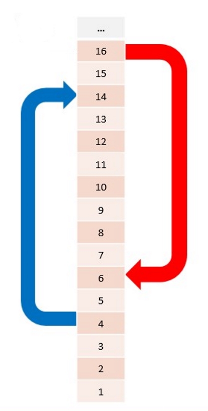
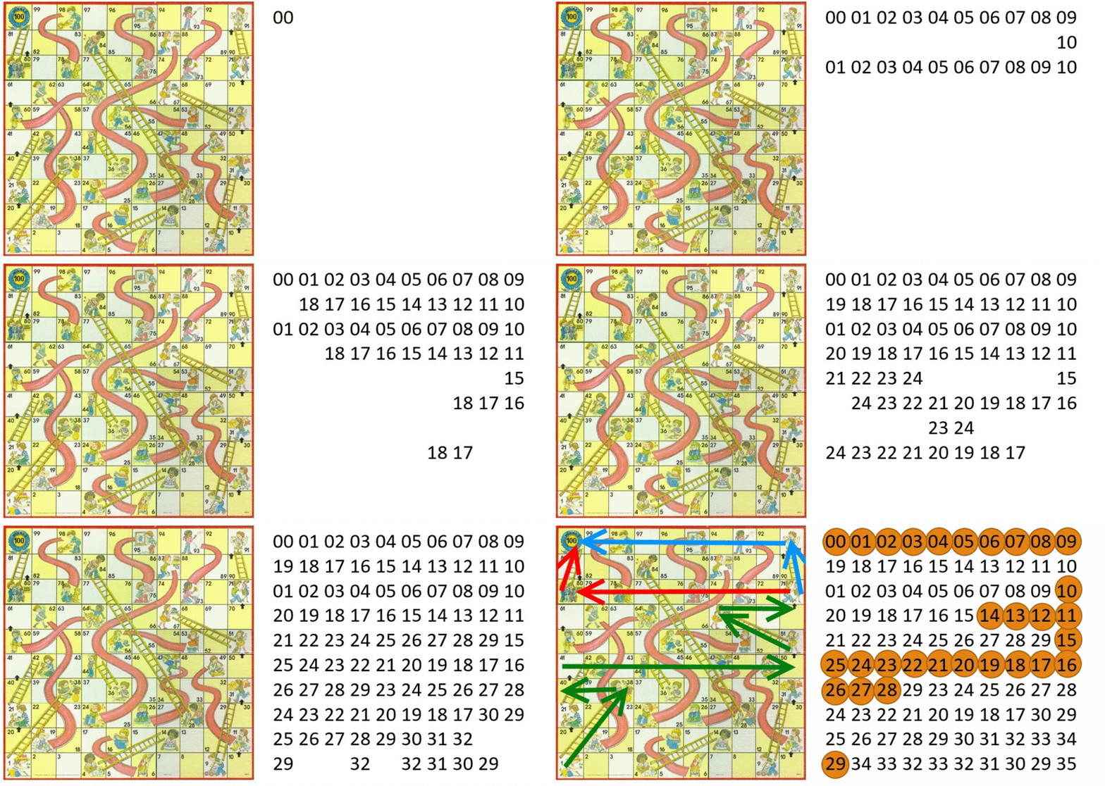
Simple Example - Chutes and Ladders
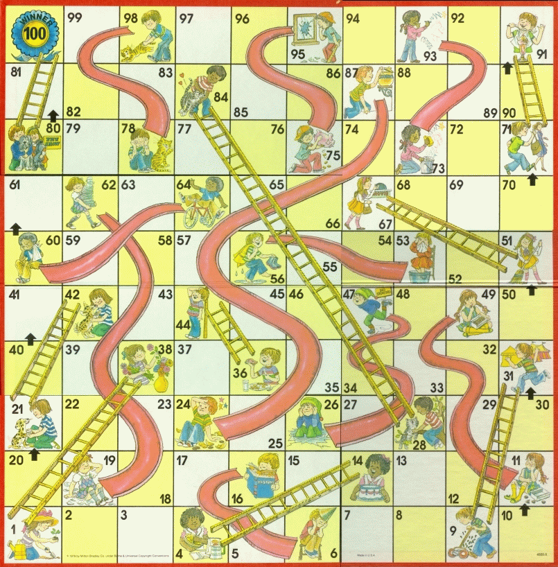
Chutes and Ladders 3.gif Linear Array.jpg

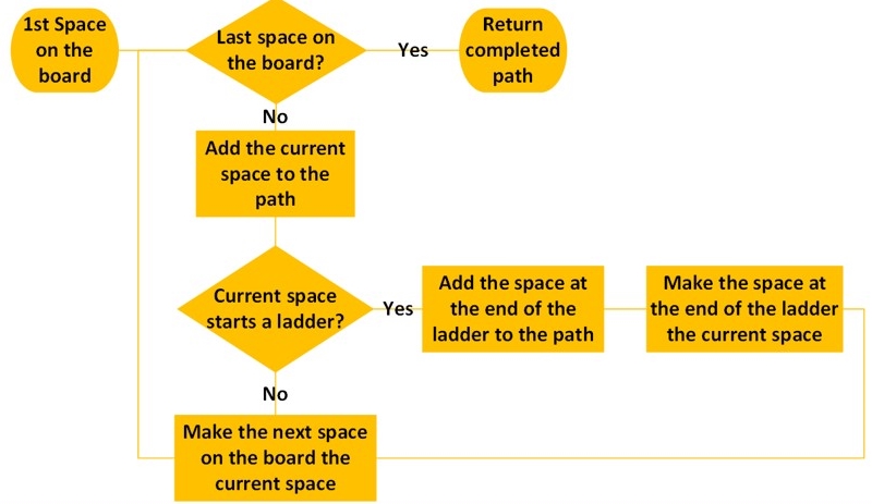
Chutes and Ladders - Greedy Algorithm

  • Start at the 1st space on the board​
  • While we haven't reached the last space​
    • Add the space to the current path​
    • If the current space has a ladder​
      • Add the end of the ladder to the path​
      • Make that space the current space​
    • Move to the next space on the board​
  • Return the completed path through the board
Greedy Algorithm.jpg

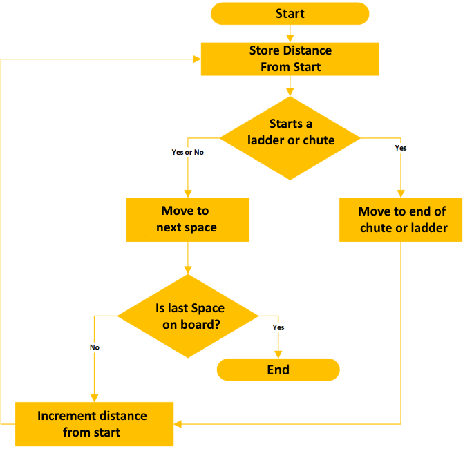
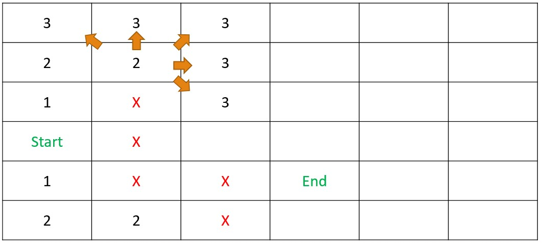
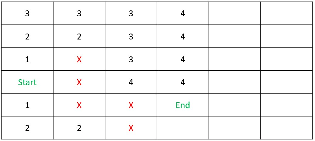
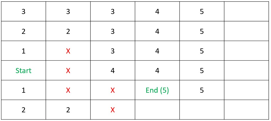
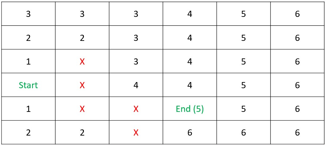
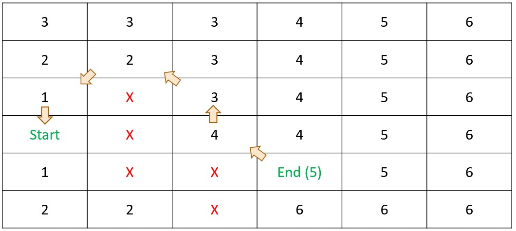
Dynamic Programming - Step 1

DetermineDistance(s,d)

  • Call DetermineDistance(space[0], 0)
  • If shorter​ than previously found
    • Set DistanceFromStart property
    • If this space starts a chute or ladder​
      • DetermineDistance(endOfNavigation, distanceFromStart+1​)
    • If not at the end of board​
      • DetermineDistance(nextSpace, distanceFromStart+1)
  • Return all spaces with their DistanceFromStart property populated
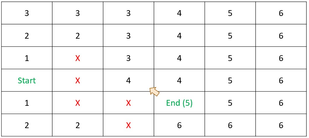
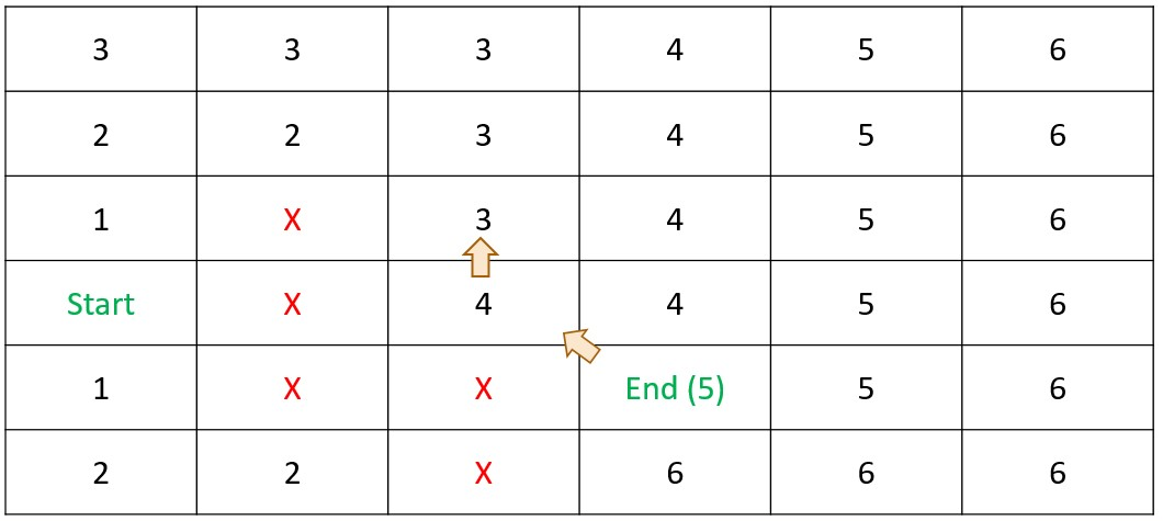
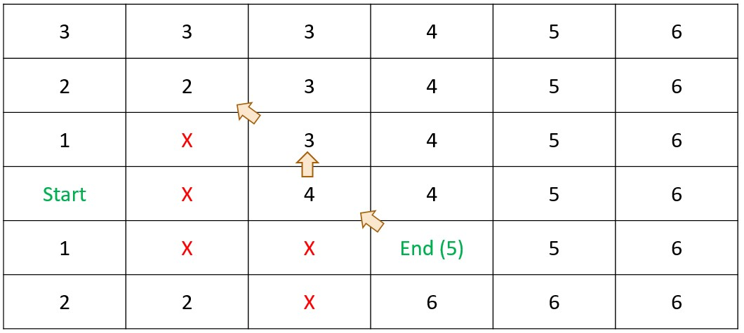
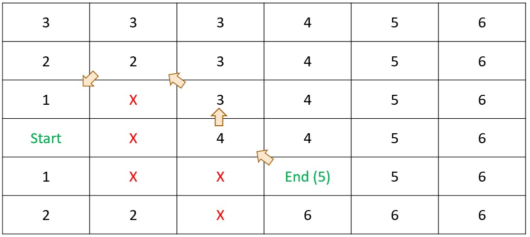
Determine Distance from Start.png

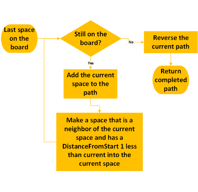
Dynamic Programming - Step 2

  • Start at the last space on the board​
  • While we are still on the board​
    • Add the current space to the path​
    • Set the current space to a space that is a neighbor of the current space and whose DistanceFromStart is space.DistanceFromStart-1​
  • Reverse the direction of the path​
Retrace Path - Smaller.png

Memoization

Memoization.gif

Shortest Path

Slide79_1000x475.jpg

Shortest Path

Slide80_1000x475.jpg

Shortest Path

Slide81_1000x475.jpg

Shortest Path

Slide82_1000x475.jpg

Shortest Path

Slide83_1000x475.jpg

Shortest Path

Slide84_1000x475.jpg

Shortest Path

Slide85_1000x475.jpg

Shortest Path

Slide86_1000x475.jpg

Shortest Path

Slide87_1000x475.jpg

Shortest Path

Slide88_1000x475.jpg

Shortest Path

Slide89_1000x475.jpg

Shortest Path

Slide90_1000x475.jpg

Summary - Dynamic Programming

  • Populate the cache​
    • Simple calculations​
    • Build from the ground-up​
  • Use the cached data to determine the answer(s)​
    • Work backwards through the cache​
  • Guaranteed Optimality​
    • A fully populated cache means all options are explored​
    • Works in any number of dimensions​
  • Works with any graph (nodes & edges)​
    • Works best when​
      • Problems can be described recursively​
      • 1 or more axis are limited in scope
DP_800x800.png

Beary - The Beary Barry Bot

Beary_600x600.png
 

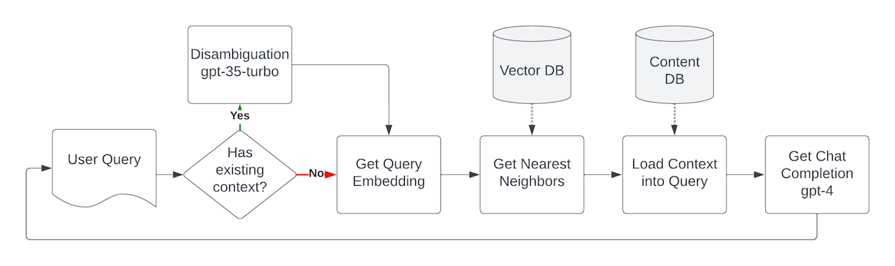
Beary Flow

Beary Demo - Flowchart - Horizontal Flow - 1280x381.png

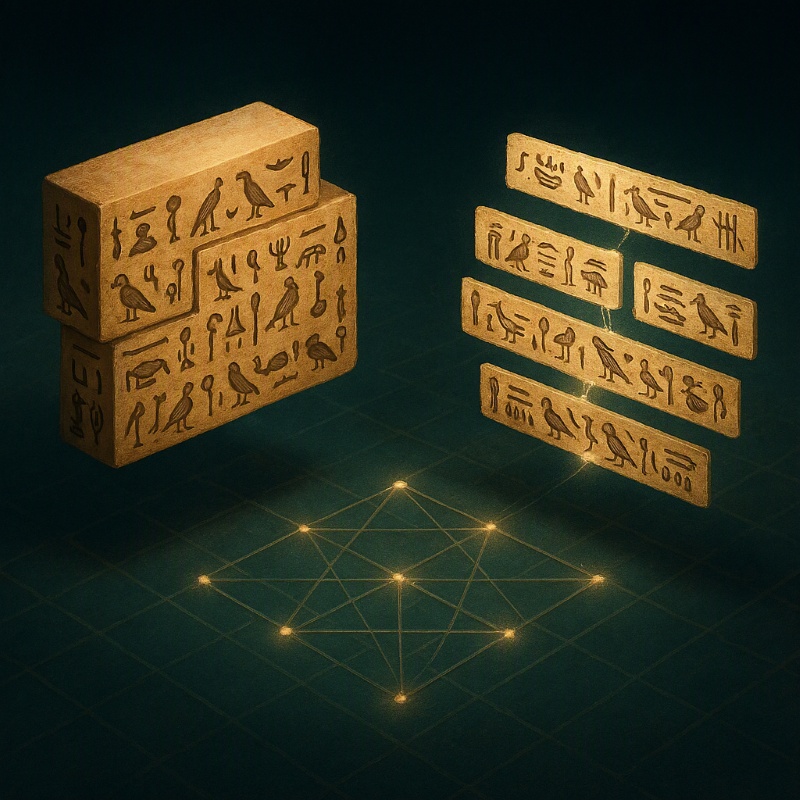
The Chunking Problem

  • Beary is chunking content inefficiently

  • We really have a segmentation problem

    • Given a paragraph, where do the boundaries belong?
  • Each candidate chunk has a quality score

    • Semantically coherent chunks > mixed-topic chunks
  • The goal is global, not local

    • Maximize the total chunk quality across the whole paragraph
  • This is the same shape as earlier DP problems

    • We are choosing an optimal partition, like shortest-path and knapsack style decisions
Chunking-800x800.png

Scoring the Chunks

  • Score each candidate chunk with a simple objective
\[ score(i,j) = avg\_similarity(i..j) - 0.1 \times (chunk\_size - 1) \]
  • High internal similarity is good

    • Sentences that belong together should raise the score
  • Bigger chunks pay a penalty

    • We do not want one oversized chunk to absorb unrelated ideas
  • This is value minus cost

    • Reward improvements to the solution
    • Penalize what bloats the solution
ChunkScoring-800x800.png

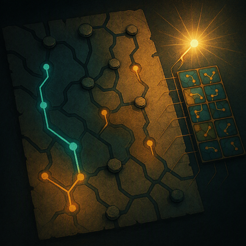
Why Dynamic Programming Applies

  • Greedy segmentation can look right and still lose

    • Local best can block a better score later
  • Brute-force segmentation is expensive over large datasets

    • Combinations grow exponentially with sentence count
  • Dynamic Programming gives optimal chunking in O(n^2)

    • Solve each suffix once and reuse it
\[ DP[i] = \max_{j \ge i} \left( score(i,j) + DP[j+1] \right) \]
  • Uses the same memoization pattern
    • State at index \(i\), try choices \(j\), cache best future value
OptimalSubstructure-800x800.png

Sample Paragraph

The clarity-first, object-oriented implementation of a Tokenizer is written in C#, my language of choice. I suspect it will be easy to have it translated into nearly any other programming language if that makes it easier to understand. The goal of this implementation is not speed, it is transparency. You can step through Encode and Decode to see exactly what is happening. The code is available on GitHub.


  1. The clarity-first, object-oriented implementation of a Tokenizer is written in C#, my language of choice.
  2. I suspect it will be easy to have it translated into nearly any other programming language if that makes it easier to understand.
  3. The goal of this implementation is not speed, it is transparency.
  4. You can step through Encode and Decode to see exactly what is happening.
  5. The code is available on GitHub.

Sentence Similarity
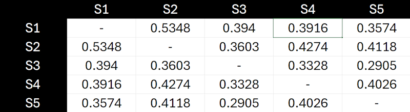
SimilarityScores_Raw_800x220.png
  1. The clarity-first, object-oriented implementation of a Tokenizer is written in C#, my language of choice.
  2. I suspect it will be easy to have it translated into nearly any other programming language if that makes it easier to understand.
  3. The goal of this implementation is not speed, it is transparency.
  4. You can step through Encode and Decode to see exactly what is happening.
  5. The code is available on GitHub.

Sentence Similarity
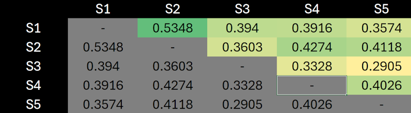
SimilarityScores_Highlighted_800x220.png
  1. The clarity-first, object-oriented implementation of a Tokenizer is written in C#, my language of choice.
  2. I suspect it will be easy to have it translated into nearly any other programming language if that makes it easier to understand.
  3. The goal of this implementation is not speed, it is transparency.
  4. You can step through Encode and Decode to see exactly what is happening.
  5. The code is available on GitHub.

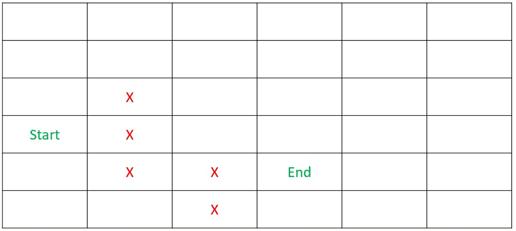
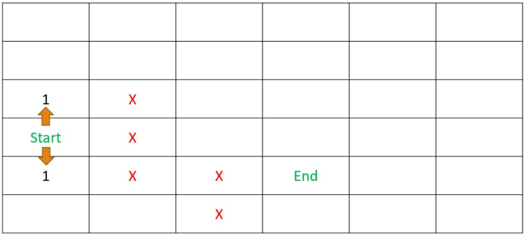
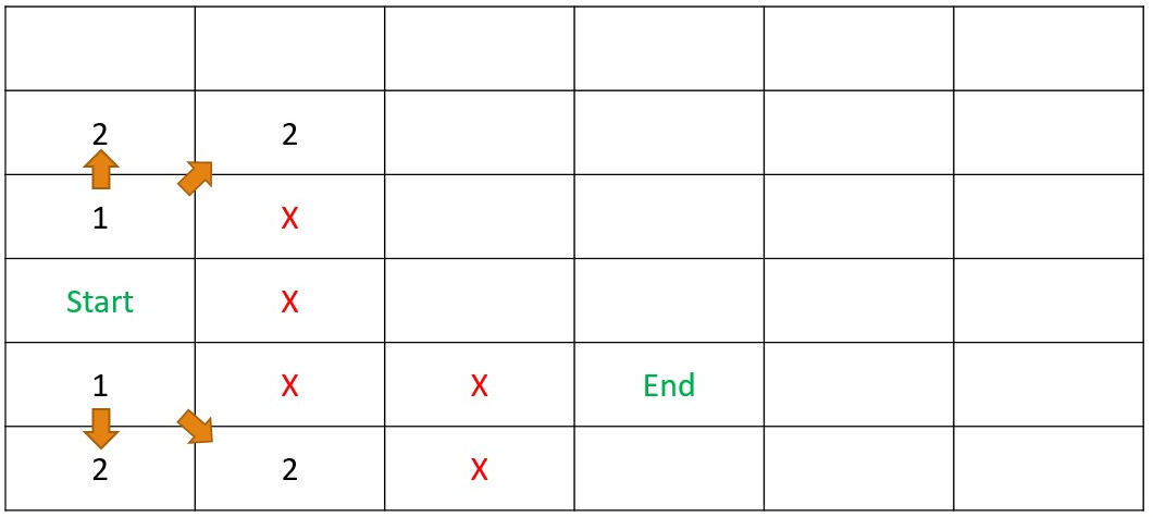
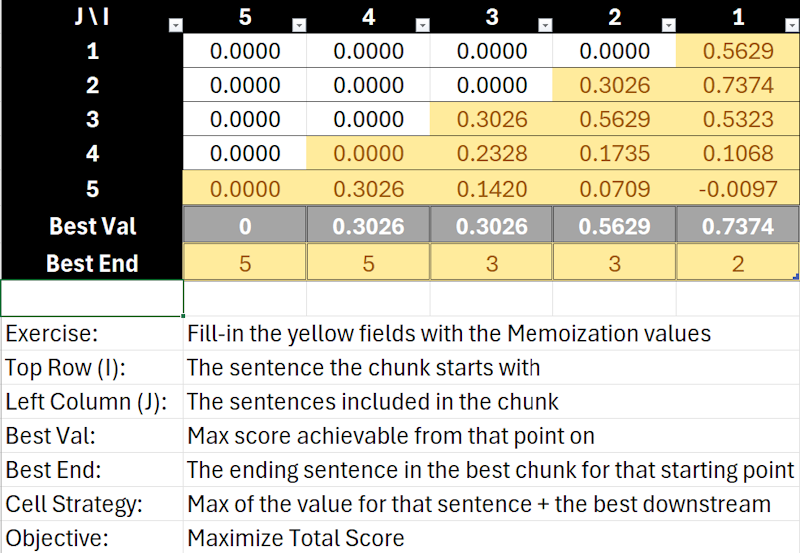
Hands-On Chunking
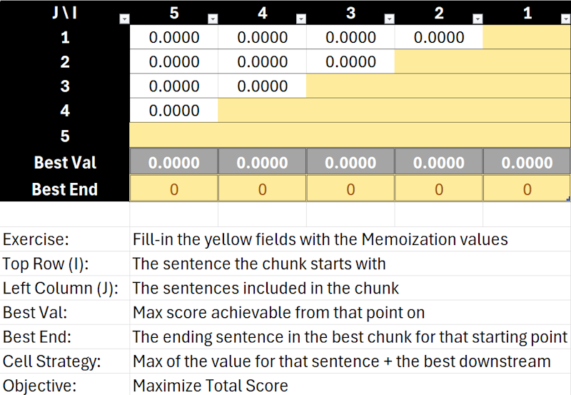
ChunkingExercise_EmptyGrid.png
  brainbreaks.png

Exercise Solution

ChunkingExercise_CompletedGrid.png

Genetic Algorithms

Find Solutions by Simulating Darwinian Evolution​

  • Each candidate solution is defined by its properties (chromosomes)​
  • A fitness function is used to determine which solutions "survive"
    • A simulation may be used as the fitness function
  • Surviving solutions may mutate and evolve other solutions​
EvolutionaryLab-800x800.png

Optimality is Never Guaranteed

  • Optimal solution may never be found
    • i.e. If a optimality requires a large combination of elements
  • Optimum may be found but not recognized
    • If conditions make that solution non-optimal at that moment
      • i.e. If a key feature is not used during the simulation
    • Minimize the liklihood by increasing simulation size
OptimalityNotGuaranteed-800x800.png

A Deep Dive into Genetic Algorithms

  • Want the full Genetic Algorithms deep dive?

  • Dedicated 1-hour session

    • Tomorrow at 10:00 AM
  • We will cover

    • DNA representation and fitness design
    • Evolution parameters and convergence tradeoffs
    • End-to-end implementation details and experimentation
GeneticAlgorithms-800x800.png

Grouping (Partitioning)

Ways to organize a collection of items into meaningful subsets

  • Classification - grouping using known categories
  • Clustering - grouping by discovering categories
Grouping-800x800.png

Classification

Grouping data into known categories based on features of each item

  • Can be used for:
    • Grouping items with shared properties together
    • Identifying which known group a new item belongs to
    • Normalization of input/output
  • Usually based on a training set of labeled data
    • The model learns the features that define each category
    • New items are classified based on learned features
    • Classification is a supervised learning problem
Classification-800x800.png

Assigning Meaningful Labels

  • Start with known labels:
    • Spam or not spam
    • Defect or no defect
    • Support ticket category
    • Image contents
  • The model is trained from labeled examples
  • Then it predicts the best label for new inputs

Shape of a Classification Problem

  • Labeled examples show the model what the right answer looks like

    • Each example includes input data plus the correct label
  • Features are the details the model is allowed to use

    • Measurements, properties, words, pixels, counts, or categories
    • Chosen because they may help separate one label from another
  • Target classes are the labels the model is allowed to predict

    • The known categories we care about
    • The output must be one of these classes
  • Training searches for a pattern from features to target class

  • Prediction applies that pattern to an unlabeled input

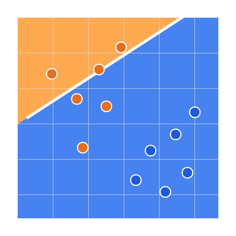
Decision Boundaries

  • A classifier divides feature space into regions

  • Each region predicts a different target class

  • The line between regions is a decision boundary

  • New inputs are classified by where they land

  • Different algorithms draw different kinds of boundaries

DecisionBoundaries-800x800.png

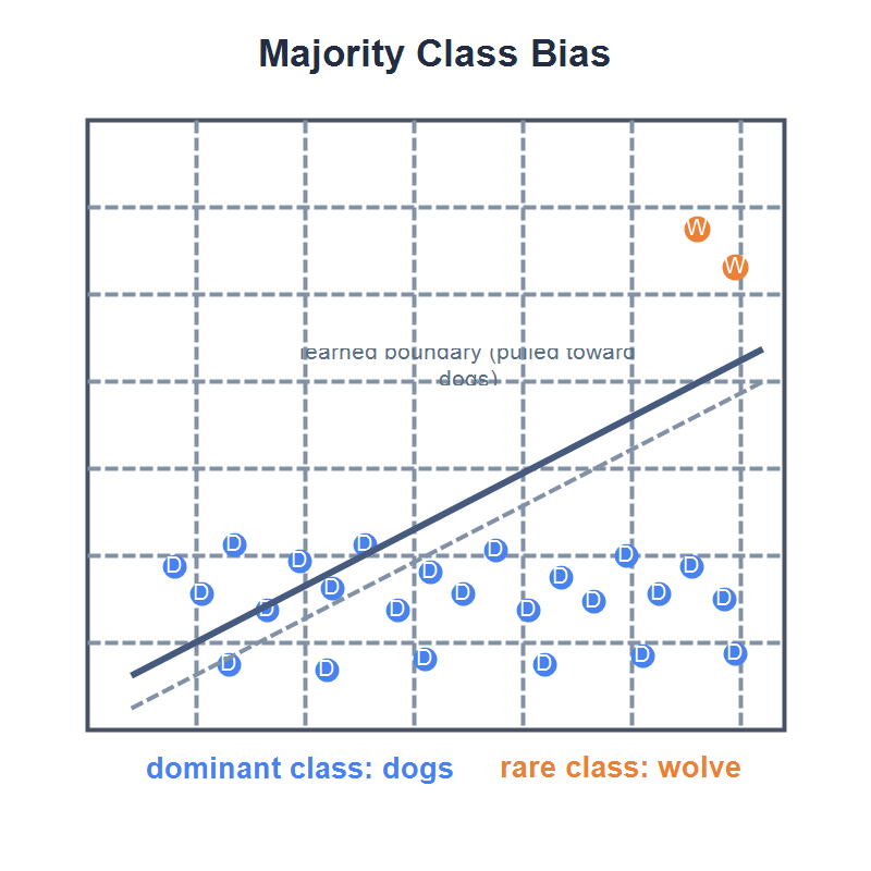
Majority Class Bias

  • Class Imbalance: one class dominates the training data

  • Majority Class Bias: model defaults to the common class

  • Example: 99% dogs, so a wolf is predicted as "dog"

  • Why: loss is optimized by being right on frequent examples

  • Fixes: class weighting, oversampling/SMOTE, undersampling, threshold tuning

MajorityClassBias-800x800.png

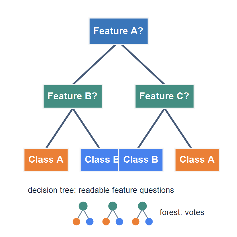
Rule-Based vs Tree-Based

  • Decision trees are readable classification models

    • Each split asks a question about a feature
    • Each branch narrows the possible class
    • Each leaf predicts a target class
    • Random forests use many trees & combine votes
      • Less explainable
      • Often generalize better
  • Rule-based classifiers

    • Explicit if/then rules
    • Usually written by people
TreeBasedClassifiers-800x800.png

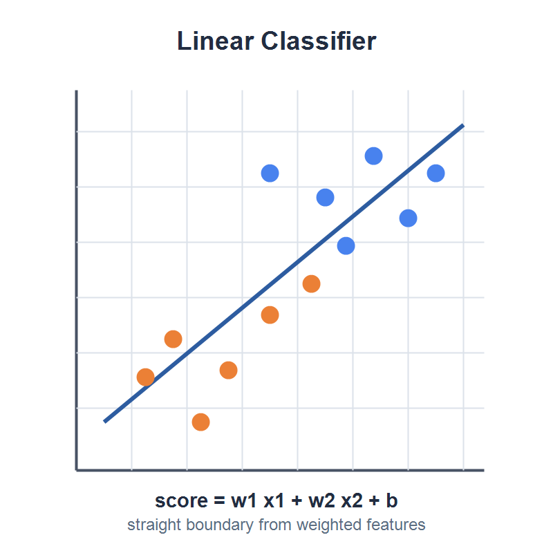
Linear Classifiers

  • Separate classes with a weighted feature score

    • Each feature contributes to the final decision
    • The boundary is a line or flat surface in feature space
  • Boundary Identification Methods

    • Logistic regression
      • Estimates the probability of a class
    • Linear SVMs
      • Support Vector Machines
      • Find the hyperplane that maximizes margin between classes
LinearClassifiers-800x800.png

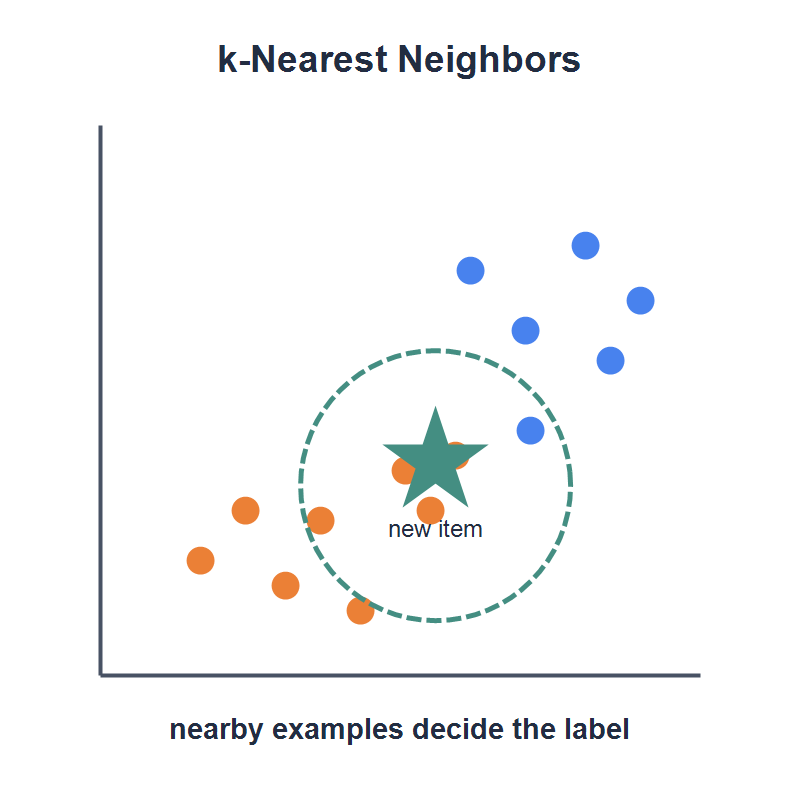
Instance-Based Classifiers

  • k-Nearest Neighbors

    • Which labeled examples are closest
    • Predicted class is the majority of neighbors
  • Nearest Centroid

    • Compute the centroid of each class
    • Predicted class is the closest centroid
  • The same concept is central in clustering

InstanceBasedClassifiers-800x800.png

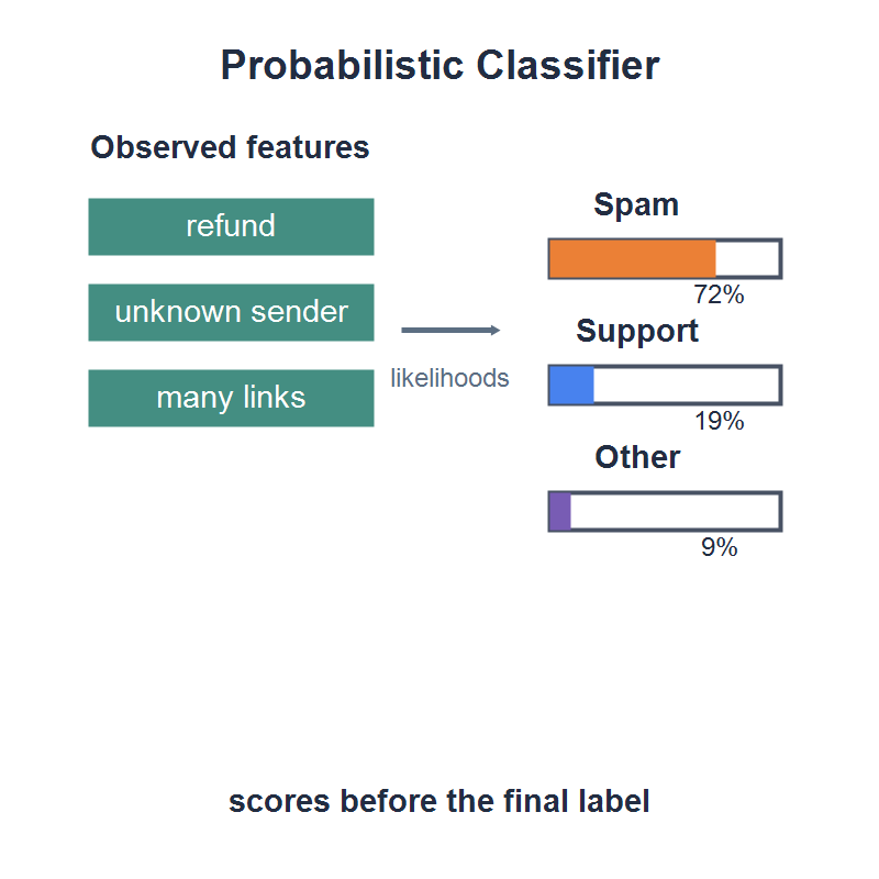
Probabilistic Classifiers

Estimate which label is most likely

  • Naive Bayes

    • Combines evidence from observed features
    • Lightweight and useful for text-like signals
    • Often used in spam detection & sentiment analysis
  • Gaussian Mixture Models (GMMs)

    • Classes modeled as a mix of distributions
    • Assumes features follow a normal distribution
    • Complicated and expensive but can be very accurate
  • In both cases output is a ranked set of class scores

  • The final label is the highest-scoring class

ProbabilisticClassifiers-800x800.png

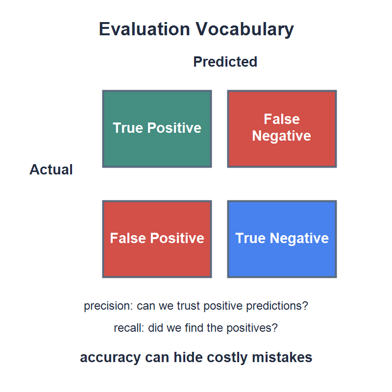
Evaluating Classification Results

Accuracy alone can hide important mistakes

  • A "confusion matrix" shows prediction vs actual
  • False positives and negatives may have different costs
    • Please no false negatives from my fire alarm
    • False positives are annoying but not dangerous
  • Precision: are positive predictions trustworthy?
    • High-Precision: Usually predicts wolves properly
    • Low-Precision: May predict wolf when just a dog
  • Recall: were the important positives found?
    • High-Recall: Usually finds all the wolves
    • Low-Recall: May miss a wolf but often correct when it predicts one
ClassificationEvaluation-800x800.png

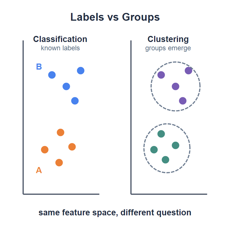
Classification vs Clustering

  • Classification starts with known target classes

    • Which known label fits this item?
  • Clustering starts without those labels

    • What groups seem to exist?
  • Both can use the same feature space

ClassificationToClustering-800x800.png

Clustering

  • Unsupervised machine learning technique
  • Clusters form around centroids (geometric center)
  • Data points are grouped based on their similarity
    • Minimize the error (distance from centroid)
  • Advantages
    • No need to define a distance threshold
  • Disadvantages
    • Quality is use-case dependent
    • Often requires the number of clusters to be specified
Clustering-800x800.png

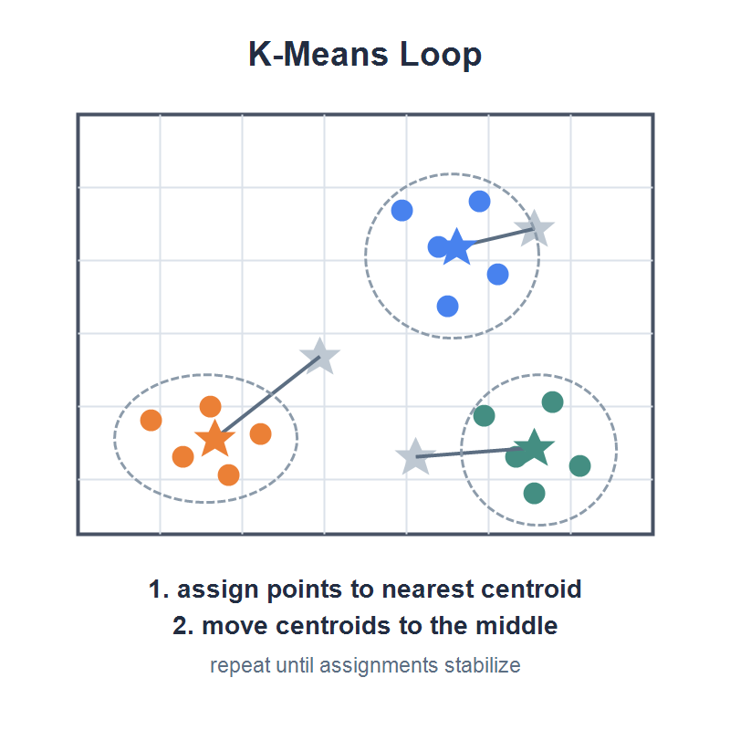
K-Means Clustering

Groups points around centroids

  • Iterative process

    • Start by choosing \(k\), the number of clusters
    • Assign each point to the nearest centroid
    • Move each centroid to the middle of its assigned points
    • Repeat until the assignments converge
  • Different \(k\) values can tell different stories

  • Use context and experimentation to determine utility

    • Quality metrics can help
KMeansLoop-800x800.png

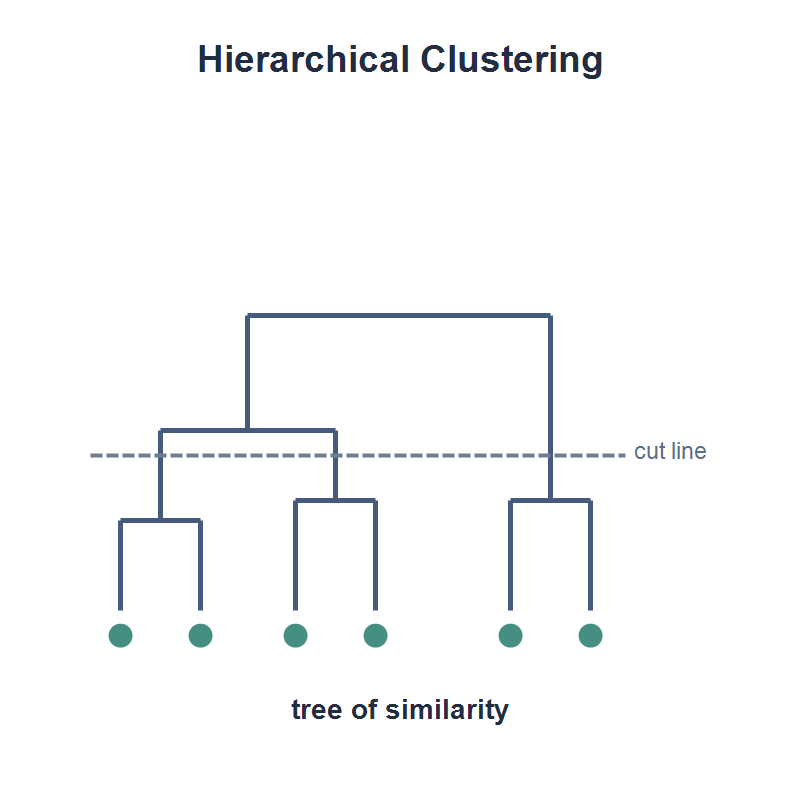
Hierarchical Clustering

Builds a similarity tree (dendogram)

  • Iterative process

    • Start with each item in its own group
    • Nearby items merge into small groups
    • Small groups merge into larger groups
  • Cutting the tree at different heights gives different cluster counts

  • Useful when the right number of groups is not obvious

HierarchicalClustering-800x800.png

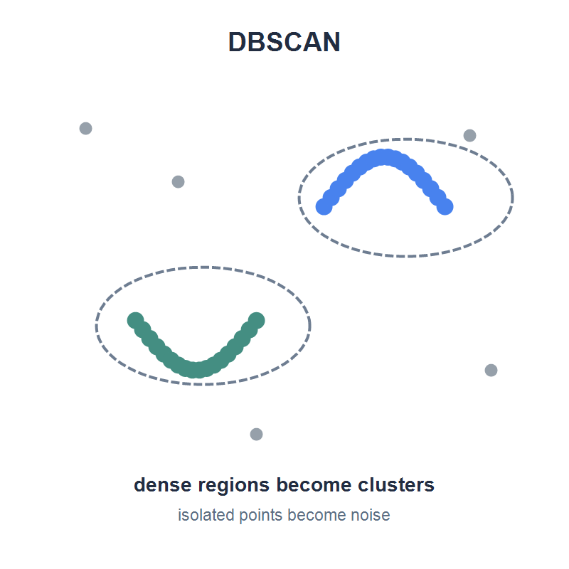
DBSCAN

Finds dense regions in feature space

  • Crowded neighborhoods become clusters
    • Clusters high density regions separated by low density
    • Does not require \(k\) up front
    • Sparse isolated points are treated as noise
  • Can find irregular shapes that k-Means misses
    • k-Means centroids assume spherical clusters
    • Mapping is a common use-case
  • Can be distributed using DDBSCAN
    • Similar to MapReduce, but with a merge step
DBSCAN-800x800.png

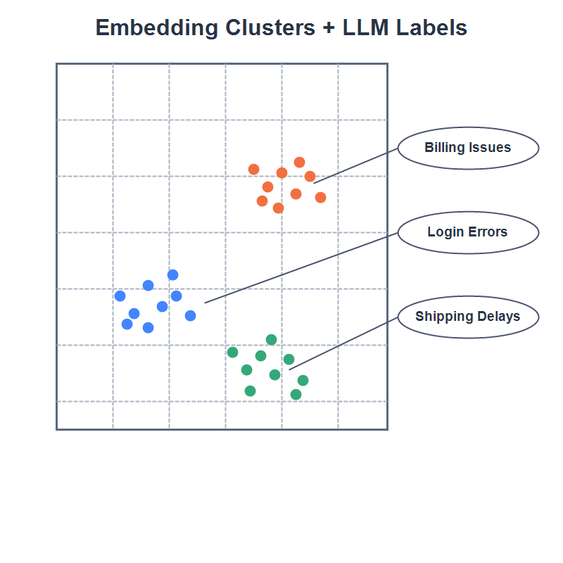
Cluster Labeling with LLMs

Clusters are groupings without meaning

  • LLMs can identify themes in textual clusters
    • Other models needed for different data types
    • Can be used on the group or on the centroid
  • Labels identify groups with usable categories
    • Unlocks routing, triage, and analytics workflows
ClusterLabelingWithLLMSummaries-800x800.png

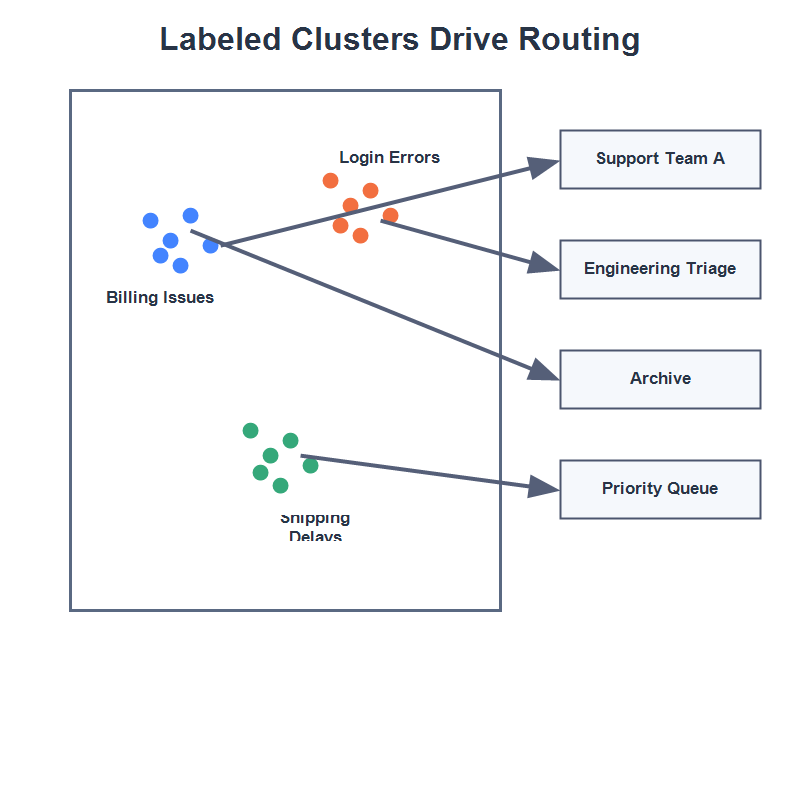
Cluster Routing for Automation

Labeled clusters become direct decision inputs

  • Routes can be mapped
    • Teams
    • Pipelines
    • Archives
    • Queues
  • Automation replaces keyword rules
    • Reduces brittleness
    • Reduces maintenance
    • Updates can be automated
ClusterRoutingForAutomation-800x800.png

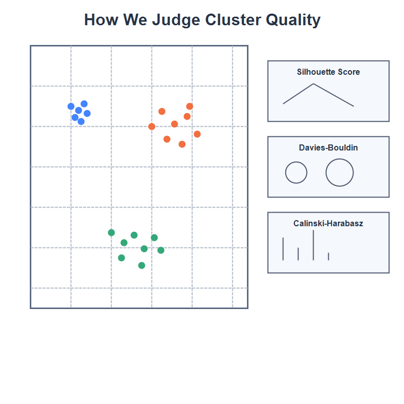
Cluster Quality Metrics

With no existing labels, we need to evaluate cluster structure directly

  • Silhouette Score
    • Higher scores: tighter clusters and better separation
    • \(\text{Silhouette} = \frac{\text{separation}}{\text{cohesion}}\)
  • Davies-Bouldin Index
    • Lower scores: less overlap and cleaner boundaries
    • \(\text{DBI} = \frac{\text{within‑cluster scatter}}{\text{between‑cluster separation}}\)
  • Calinski-Harabasz Score
    • Higher scores: clusters more tighter and more separated
    • \(\text{CH} = \frac{\text{between‑cluster variance}}{\text{within‑cluster variance}}\)
ClusterQualityMetrics-800x800.png

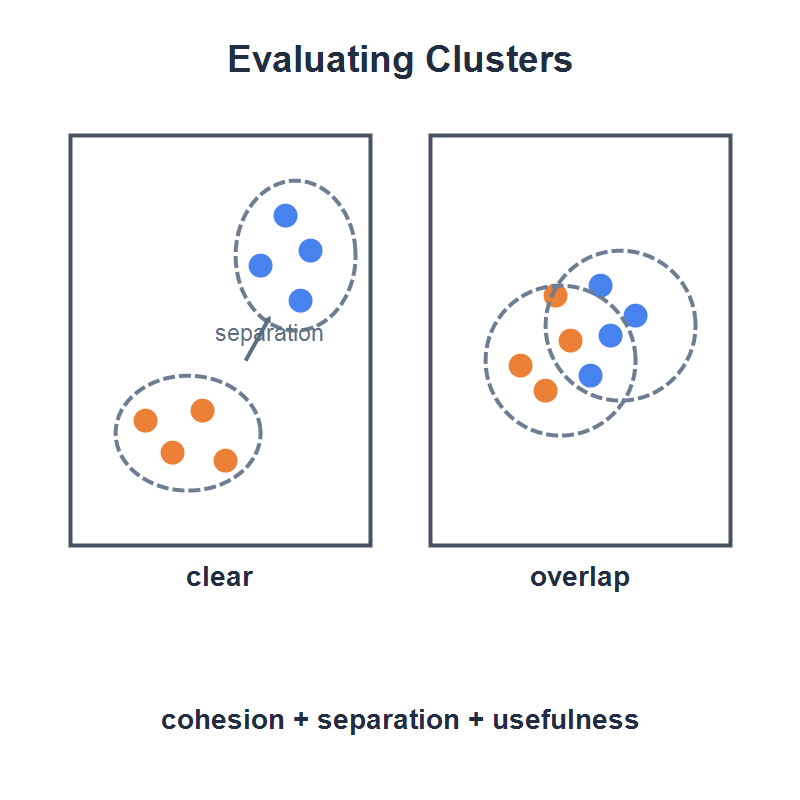
Evaluating Clustering Results

Good scores \(\neq\) fitness for purpose

  • Evaluation is about whether the grouping is useful
    • Will the grouping help the real task?
  • Good clusters are:
    • Cohesive internally
    • Separated from each other
    • Interpretable and actionable
    • Useful for our needs
ClusteringEvaluation-800x800.png

Use-Case: Semantic Distance

semantic-dna-surreal 800x800.jpeg

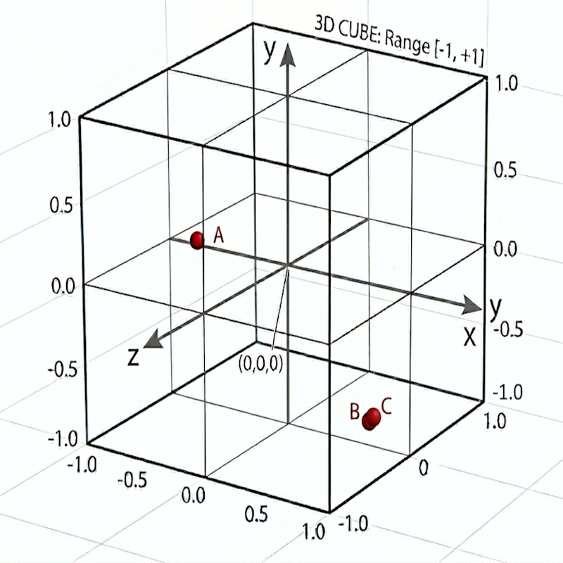
Embeddings

  • A point in multi-dimensional space
  • Mathematical representation of a word or phrase
  • Encode both semantic and contextual information

  • Model: text-embedding-ada-002
  • Vectors normalized to unit length
  • Use 1536 dimensions
VectorSpace3D.png

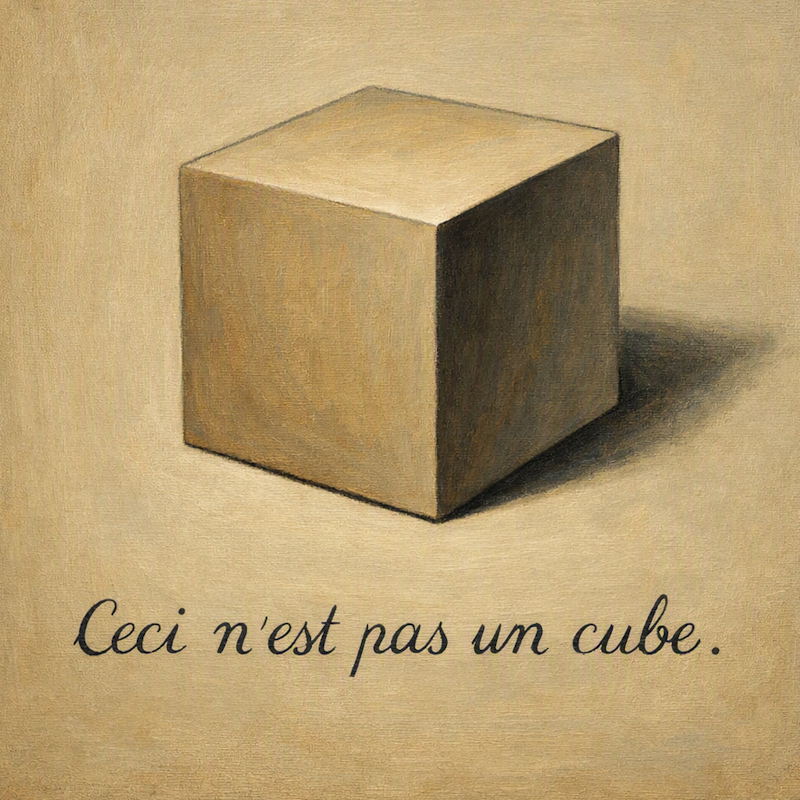
3-D Space Projected into 2-D

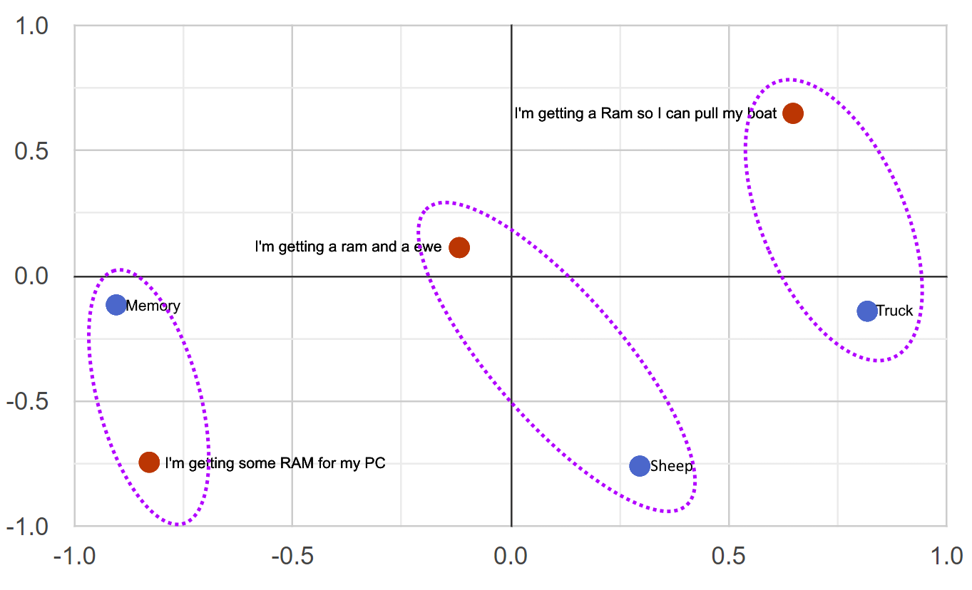
Necker_cube_with_background.png
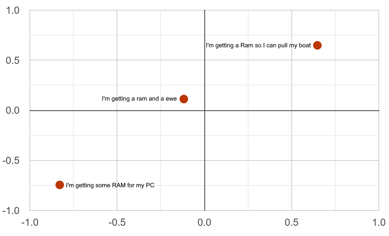
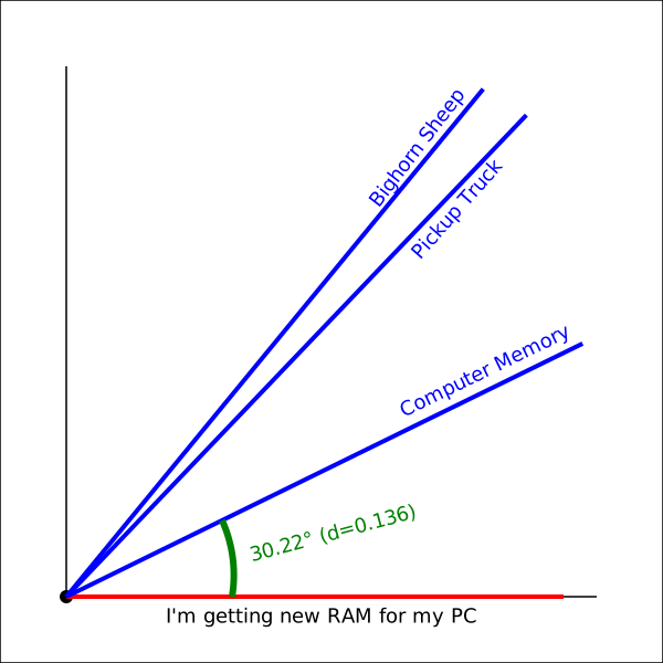
  Ram - Just Statements.png
  Ram - With Clusters.png

Embedding

Creating Order from Chaos

  • Unstructured string => Structured float[]
  • Allows mathematical operations
    • Cosine Similarity & Distance
    • Nearest Neighbor Search
    • Clustering
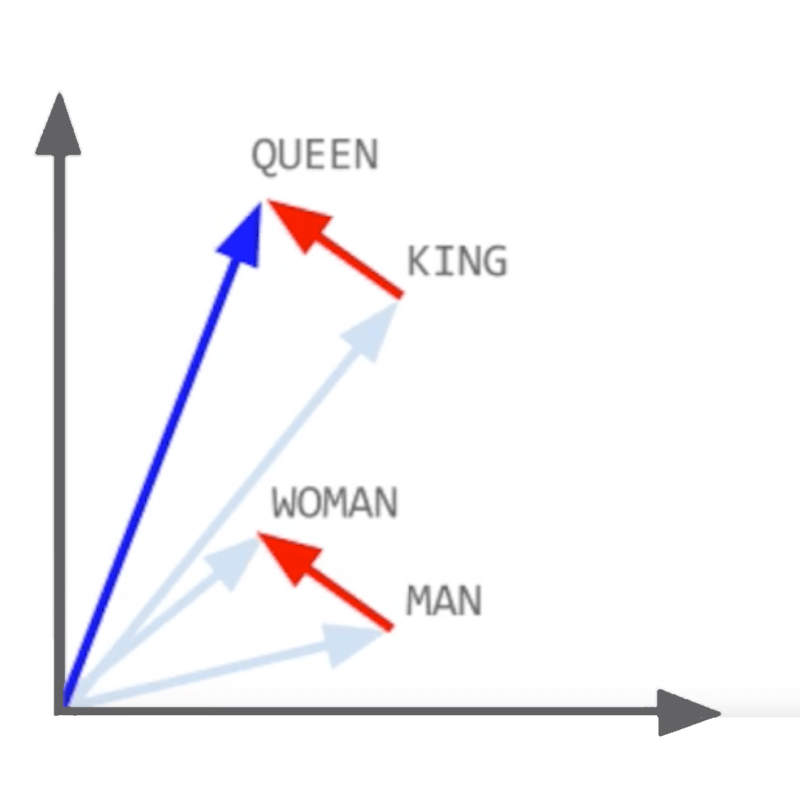
    • Vector Addition & Subtraction
    • Dimensionality Reduction (e.g., PCA)
    • Anomaly Detection
VectorRelationships-QueenToKing-WomanToMan.png

Cosine Similarity & Distance

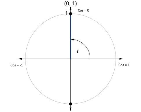
Relate vectors based on the angle between them

  • Cosine Similarity ranges from -1 to 1, where:

    • +1 indicates that the vectors represent similar semantics & context
    • 0 indicates that the vectors are orthogonal (no similarity)
    • -1 indicates that the vectors have opposing semantics & context
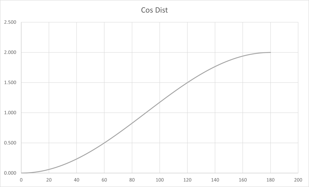
  • Cosine Distance is defined as 1 - cosine similarity where:

    • 0 = Synonymous
    • 1 = Orthogonal
    • 2 = Antonymous

Note: For normalized vectors, cosine similarity is the same as the dot-product

Cosine Unit Circle - Enhanced.jpg

Cosine Distance

Cosine Distance 989x600.png

Cosine Distance

Angles2.svg

Embedding Distance

Feature Example
Synonym "Happy" is closer to "Joyful" than to "Sad"
Language "The Queen" is very close to "La Reina"
Idiom "He kicked the bucket" is closer to "He died" than to "He kicked the ball"
Sarcasm "Well, look who's on time" is closer to "Actually Late" than "Actually Early"
Homonym "Bark" (dog sound) is closer to "Howl" than to "Bark" (tree layer)
Collocation "Fast food" is closer to "Junk food" than to "Fast car"
Proverb "The early bird catches the worm" is closer to "Success comes to those who prepare well and put in effort" than to "A bird in the hand is worth two in the bush"
Metaphor "Time is money" is closer to "Don't waste your time" than to "Time flies"
Simile "He is as brave as a lion" is closer to "He is very courageous" than to "He is a lion"

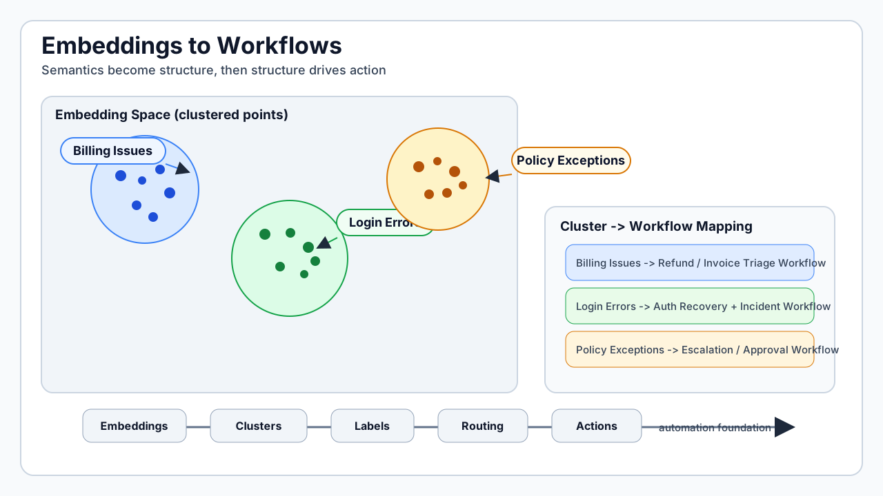
Embeddings to Workflows

  • Embeddings: place similar statements close together
  • Clustering: group them into meaningful categories
  • LLMs: can label each cluster
  • Routing: new statements to the best cluster
  • Actions: each cluster maps to a workflow

  • \(\text{text}➝\text{embedding}➝\text{cluster}➝\text{label}➝\text{routing}➝\text{action}\)
  • Clustering is the structural bridge from text to automation
Embeddings-To-Workflows-1280x720.svg

Exercise: k-Means Clustering

Goal: To see unsupervised structure emerge from embeddings using clustering

  • Download the code for k-Means clustering from GitHub
  • Review the axioms.js data file
  • Review the k-Means loop
  • Review the quality scoring code
  • Run the code to create 4 clusters
    • Review the Representative axioms for each cluster
    • Review the quality scores
  • Choose a different \(k\) and rerun
    • See how cluster structure changes
AIDemos-Clustering-QR-800.png
  brainbreaks.png

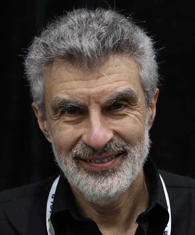
AI ≠ ML ≠ LLMs

  • LLMs are one kind of learning model
  • Learning models are one kind of AI model
  • Logic, search, optimization, and planning are often AI

Image: Yoshua Bengio by By Xuthoria

Yoshua_Bengio_663x800.jpg

AI Simulates A Rational Actor

Attempts to make the best possible decision​ based on the model and the data

  • Model - Our description of the problem
  • Data - Our understanding of the state of the domain
A Rational Actor 800x800.jpeg

Types of AI Models

  • Logic​al - Reducible to conditionals​
    • Object Oriented​
    • Rules Engine
  • Search/Optimization - Reduce and Search the Solution Space
    • Dynamic Programming​
    • Constraint Programming
  • Probabilistic/Learning - Predicts best solution from earlier data
    • Neural/Bayesian Networks
    • Genetic Algorithms

Optimization

Finding the best available solution to a problem by minimizing or eliminating undesirable factors and maximizing desirable ones.

training_animation.gif

Feasibility Problems

  • Find the best values for a set of decision variables that
    • Satisfies all constraints

Optimization Problems

  • Find the best values for a set of decision variables that​
    • Satisfies all constraints
    • Maximizes the features we want​
    • Minimizes the features we don’t want
 

Feasibility vs Optimization

  • Feasible Solutions
    • 7 Mixed Fruit
    • 1 Mixed Fruit , 2 Hot Wings, 1 Sampler Plate
  • Possible Optimizations
    • Minimize # of any single item
    • Maximize total # of distinct items
  • Possible Relaxation
    • Offer discount to relax constraint
    • Convert = to >= resulting in more feasible solutions
    • Maximize Profit

Constraint: A Required Condition

  • As an entity, constraints do 2 things

    • Verify feasibility (is there a solution that satisfies this constraint?)
    • Prune the search space (more on this coming up)
  • Infeasibility

    • Solution does not satisfy 1 or more constraints
      • Previous decisions that led to this point may need to be revisited
    • Problem has no feasible solutions
      • Relaxations may be available to find a “good-enough” solution

Types of Constraints

  • Inequality Constraints
    • \(X_1 <> 4.5\) or \(X_1 + 4X_2 < 24.0\)
  • Integer Constraints
    • Counter-intuitively, they can be harder to find solutions for
    • \(X_1 + 4X_2 < 24 \quad\text{with}\quad X_1, X_2 \in \{1,\dots,n\}\)
  • Global Constraints
    • Special “pre-defined” constraints that have a polynomial-time algorithm
      • i.e. AllDifferent Constraint
    • There are more than 400 Global Constraints known today
    • Defining these constraints using polynomial algorithms is an active research area

Objective: A Goal for the Solution

  • Objective Function

    • Equation describing how to improve a solution
    • Specify what to minimize or maximize to produce the best result
  • Specified as a goal relative to an equation

    • \(\max 3X_1 + 9X_2 \text { subject to } c_n\)
    • \(\min \sum_{i=1}^{n} A_i X_i\)
  • One objective per Model

    • Combine features by creating a "score"

Constraint Programming Models
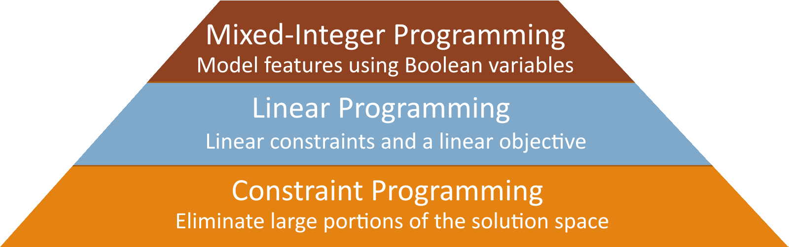
ConstraintProgrammingTypesPyramid.png

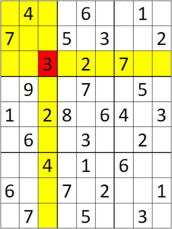
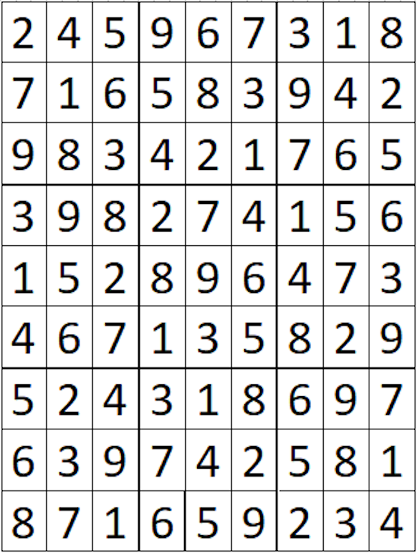
Sudoku

  • A Combinatorial Puzzle
    • 9x9 grid
    • Each row, column and 3x3 region contains [1 to 9]
  • AllDifferent constraints
    • With values restricted to integers [1 to 9]
    • 27 Constraints in total (9 rows, 9 columns, 9 regions)
01 - Sudoku Constraints - 603x800.png

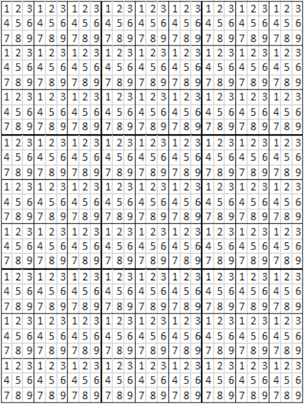
Sudoku Solution Space

  • Solution Space (aka Search Space or Feasibility Set)

    • All values that satisfy the constraint(s)
  • The solution space for a 9x9 grid is inconceivably large

    • Roughly \(2 \times 10^{77}\) possible solutions
    • At 1 Trillion per second it would take \(6 \times 10^{57}\) years
  • Even with the AllDifferent constraint, its \(6.7 \times 10^{21}\)

    • Naïve (brute-force) methods are not practical
02 - Sudoku Solution Space - 603x800.png

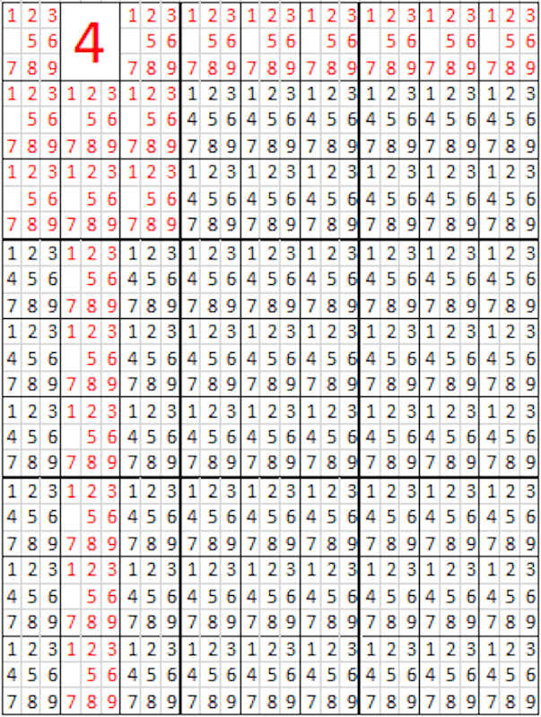
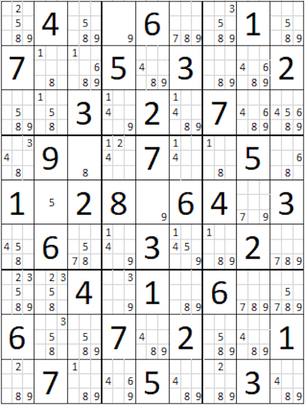
Pruning the Solution Space

  • Using constraints, we can reduce the possibilities
  • Each new learning adds new constraints

  • Question: How do we check for feasibility here?
03 - Pruning the Solution Space 01 - 603x800.png

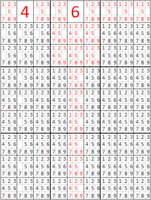
Pruning the Solution Space

  • Possible solutions: \(5 \times 10^{73}\)

    • Search space reduced by 4 orders-of-magnitude
    • Roughly 10K Possibilities Eliminated
  • Let's jump ahead

    • All of the values we've been given are filled-in
04 - Pruning the Solution Space 02 - 603x800.png

Pruning the Solution Space

  • All starting info filled-in
    • Search space pruned appropriately
    • Possible solutions: \(4 \times 10^{21}\)
    • Eliminating 56 orders of magnitude
  • We're not nearly done yet
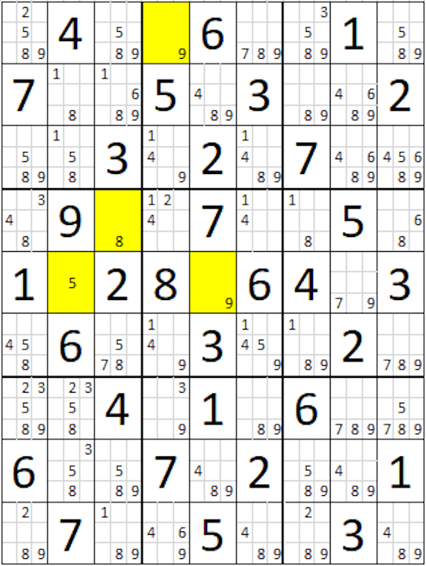
    • Look closely at the remaining options
05 - Pruning the Solution Space 03 - 603x800.png

Pruning the Solution Space

  • The reduction of search options
    • "Fixed" the value of 4 cells
06 - Pruning the Solution Space 04 - 603x800.png

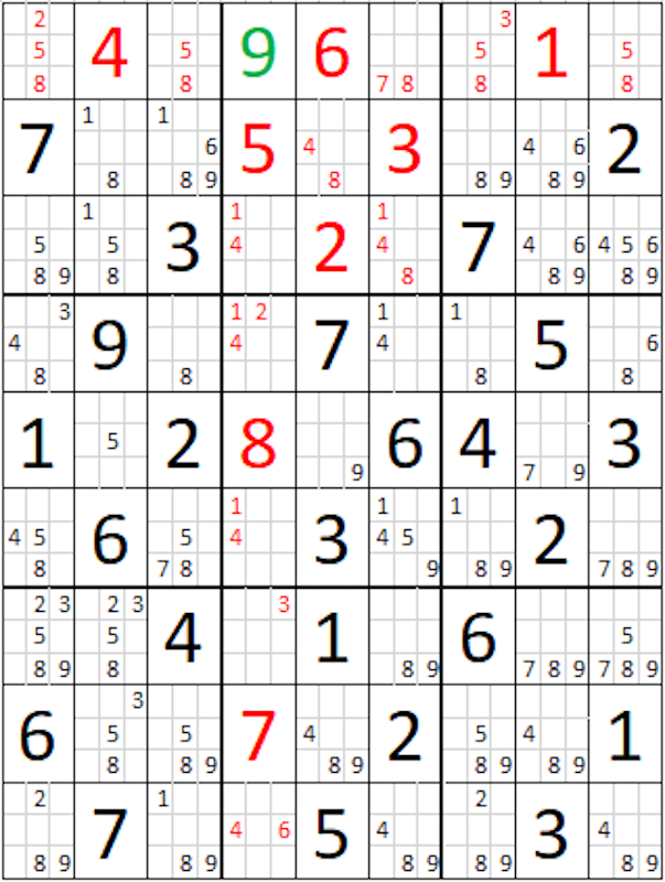
Propogation of Constraints

  • Adding info means we learn even more
    • We can reduce the search space further
  • Possible solutions: \(2 \times 10^{20}\)
07 - Pruning the Solution Space 05 - 603x800.png

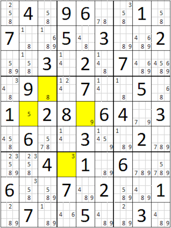
Propogation of Constraints

  • We now have even more "fixed points"
  • We continue to iteratively propagate constraints
    • Known as a "Fixed-Point Algorithm"
  • Let's jump ahead to completion of the propagation
08 - Pruning the Solution Space 06 - 603x800.png

Propogation of Constraints

  • Possible solutions: 1
  • “Guesses” Required: 0
    • Only solution was apparent after propagation
  • CSPs are not always this easy
    • Many require some form of search
09 - Pruning the Solution Space 07 - 603x800.png

Constraint Programming Pattern

  • Constraint Programming is about narrowing choices

    • Model the valid states of the problem
      • Variables, domains, and required conditions
    • Let constraints prune impossible choices
      • Every new constraint removes possible solutions
    • Search what remains until a feasible answer is found
  • LP and MIP build on the same idea

    • Constraints still define the feasible region
    • An objective chooses the best feasible answer
    • Linear structure gives us specialized algorithms

Optimization Use-Case

Determine the ideal production targets for Pete's Pottery Paradise

PetesPotteryParadise-800x800.png

Use Case: Production Targets

  • Products​
    • Small Vase​
      • 1 oz. clay, 1 oz. glaze​
      • Sells for $3.00 each​
    • Large Vase​
      • 4 oz. clay, 2 oz. glaze​
      • Sells for $9.00 each​
  • Inventory​
    • Clay - 24 oz.​
    • Glaze - 16 oz.​
  • Goal
    • Maximize Revenue

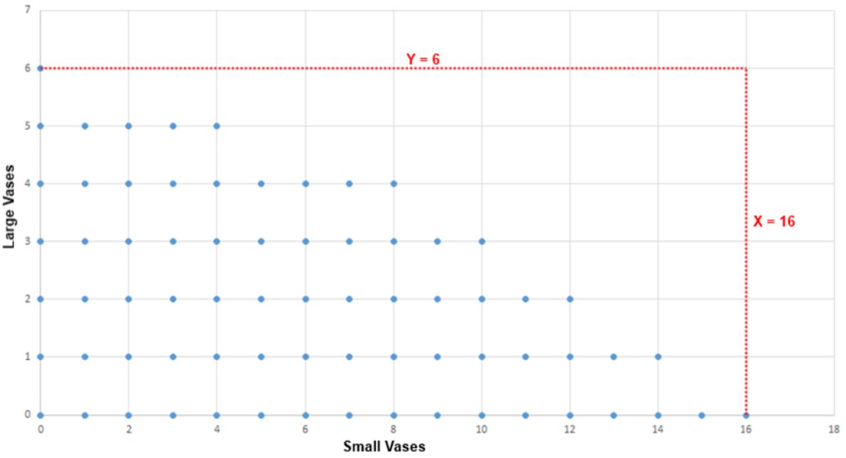
Solution Space

Solution Space Graph - With Feasible Solutions.png

Constraint Equations

  • Clay Constraint

    • \(X + 4Y \le 24 \quad \text{with} \quad X \in \{0\dots24\},\; Y \in \{0\dots6\}\)
  • Glaze Constraint

    • \(X + 2Y \le 16 \quad \text{with} \quad X \in \{0\dots16\},\; Y \in \{0\dots8\}\)

Feasible Region
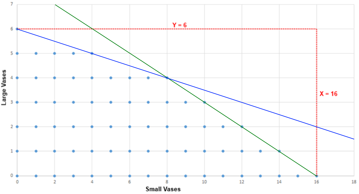
Solution Space Graph - With Feasible Solutions and Constraint Lines.png

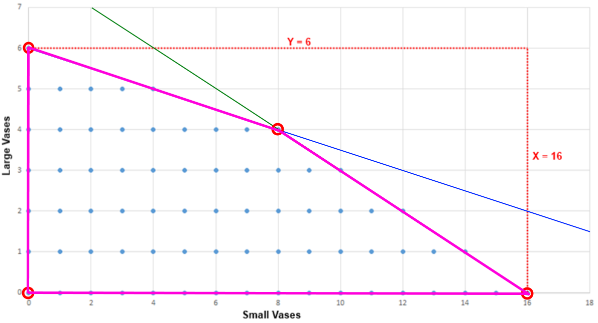
Linear Programming - Polytope

Solution Space Graph - With Polytope.png

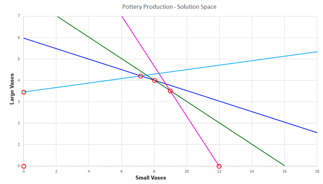
Additional Constraints

Solution Space Graph - New Polytope - 1132x645.png

The Simplex Algorithm

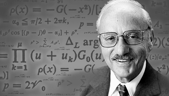
  • Created by George Dantzig in 1947
  • Built to solve linear programming problems
    • Allocate scarce resources under constraints
  • Searches the vertices of the feasible region
    • Usually far fewer places than every possible solution
  • Still used inside modern optimization solvers
    • Planning, routing, scheduling, logistics, finance
george-bernard-dantzig.jpg

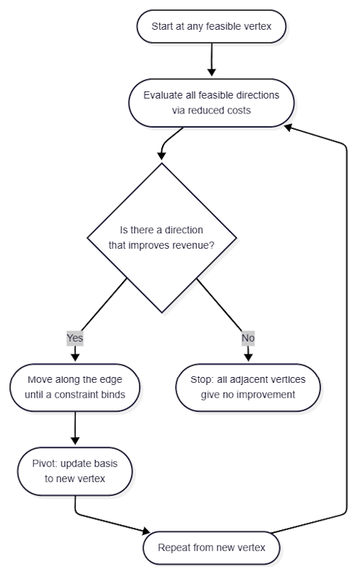
Walk the Vertices

Simplex turns optimization into a short guided walk

  • Start at any feasible vertex
    • Determine direction that improves revenue fastest
    • Move along an edge until a constraint stops you
  • Pivot to the new axis
    • Repeat from the new vertex
  • Stop when every neighboring vertex is worse
SimplexAlgorithm.png

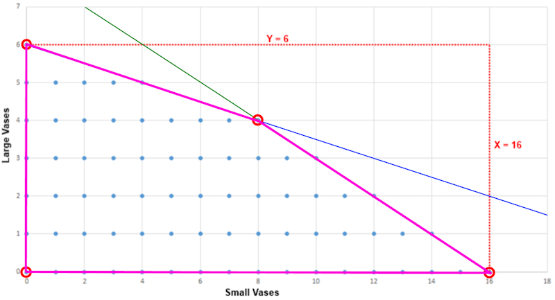
One Pivot

  • Start: (0 small, 0 large) -> revenue $0
  • Enter: make large vases first
    • They add $9 each, so revenue rises quickly
  • Leave: clay becomes the limiting constraint
    • 24 oz clay / 4 oz per large = 6 large
  • New corner: (0 small, 6 large) -> revenue $54
  • Pivot: trade along the clay edge
    • Stop at (8 small, 4 large) when glaze also binds
  • No adjacent corner improves revenue -> optimum $60
Solution Space Graph - With Polytope-800x433.png

Scheduling Use-Case

Determine the best schedule for talks at a conference

ConferenceScheduling-Photo-800x800.png

Conference Schedule

  Room 1 Room 2 Room 3
Slot 1 Session 1 Session 2 Session 3
Slot 2 Session 4 Session 5 Session 6
Slot 3 Session 7 Session 8 Session 9
Slot 4 Session 10 Open Open

LP Model - Variables

  Room 1 Room 2 Room 3
Slot 1 Session 1 Session 2 Session 3
Slot 2 Session 4 Session 5 Session 6
Slot 3 Session 7 Session 8 Session 9
Slot 4 Session 10 Open Open

  • \(X_{t,r}\)
    • \(t\) is the id of the timeslot
    • \(r\) is the id of the room
    • \(X_{t,r} \in \mathbb{Z}\) is the session id assigned to timeslot \(t\) in room \(r\)
      • \(\mathbb{Z}\) is the set of all session ids

LP Model - Constraints

  Room 1 Room 2 Room 3
Slot 1 Session 1 Session 2 Session 3
Slot 2 Session 4 Session 5 Session 6
Slot 3 Session 7 Session 8 Session 9
Slot 4 Session 10 Open Open

  • Each room/timeslot combination can have no more than 1 session
  • Each session must be scheduled exactly once
  • What if session 7 & 9 are the same speaker?
    • Desired rule: \(slot(7) \ne slot(9)\)
    • But \(X_{t,r}\) stores a session id, not a timeslot for a session
    • This requires a lookup: "where is session 7 scheduled?"
    • That lookup is not naturally a linear expression

MIP Model - Variables

Session 1 Room 1 Room 2 Room 3
Slot 1 0 0 0
Slot 2 0 0 0
Slot 3 0 1 0
Slot 4 0 0 0

Session 2 Room 1 Room 2 Room 3
Slot 1 1 0 0
Slot 2 0 0 0
Slot 3 0 0 0
Slot 4 0 0 0

Session 3 Room 1 Room 2 Room 3
Slot 1 0 0 0

MIP Model - Variables

Session 1 Room 1 Room 2 Room 3
Slot 1 0 0 0
Slot 2 0 0 0
Slot 3 0 1 0
Slot 4 0 0 0

  • \(X_{t,r,s}\)
    • \(t\) is the id of the timeslot
    • \(r\) is the id of the room
    • \(s\) is the id of the session
    • \(X_{t,r,s}\) is \(1\) if \(s\) is the session id assigned to timeslot \(t\) in room \(r\)

MIP Model - Constraints

Session 1 Room 1 Room 2 Room 3
Slot 1 0 0 0
Slot 2 0 0 0
Slot 3 0 1 0
Slot 4 0 0 0

  • Each session must be scheduled exactly once
    • \(\sum_t \sum_r X_{t,r,s} = 1 \quad \forall s\)
  • Each room/timeslot combination can have no more than 1 session
    • \(\sum_s X_{t,r,s} \le 1 \quad \forall t,r\)
  • Sessions 7 and 9 cannot be scheduled in the same timeslot
    • \(\sum_r X_{t,r,7} + \sum_r X_{t,r,9} \le 1 \quad \forall t\)

MIP Model - Objective

Session 1 Room 1 Room 2 Room 3
Slot 1 0 0 0
Slot 2 0 0 0
Slot 3 0 1 0
Slot 4 0 0 0

Create a score that improves with the desirability of the solution

  • Factors might include
    • Reduce # of different rooms in a track
    • Reduce the # of timeslot conflicts between sessions in a track
    • Reduce total steps between sessions of a track
    • Reduce distance (time & room) between multi-part sessions
    • Reduce # of different days a speaker speaks

MIP Model - Objective Example

Session 1 Room 1 Room 2 Room 3
Slot 1 0 0 0
Slot 2 0 0 0
Slot 3 0 1 0
Slot 4 0 0 0

Maximize # of sessions in the same room with Sessions 2 & 4 (a track)

  • For each Room:
    • \(\max \sum_r \left(\sum_t X_{t,r,2}\right)\left(\sum_t X_{t,r,4}\right)\)
      • If they are in the same room, the total will be 1
      • If they are in different room, the total will be 0

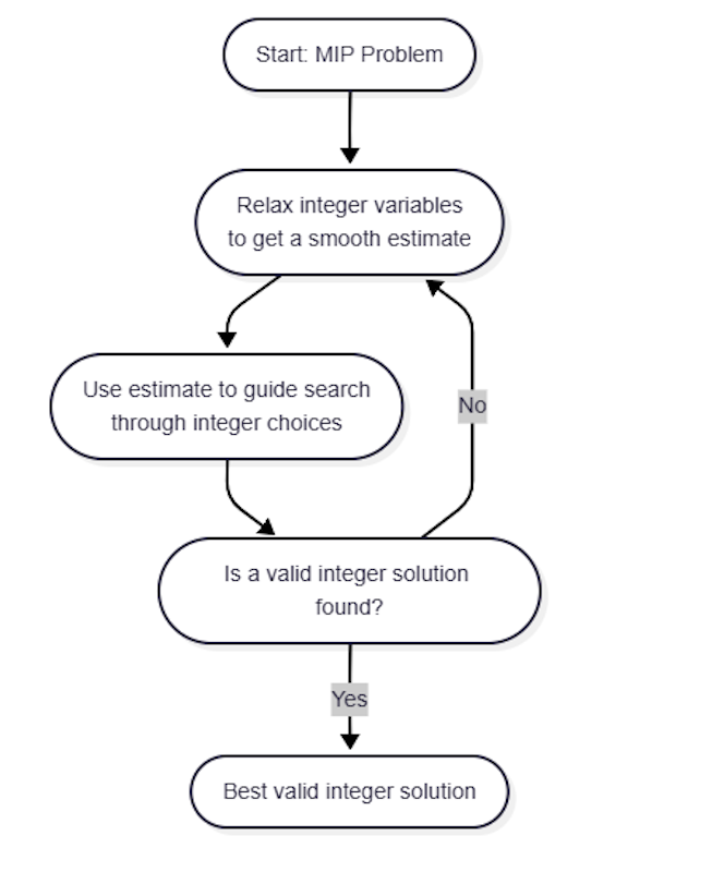
Simplex for MIP

  • Relax the constraints:

    • Boolean vars → continuous vars \(\in [0,1]\)
    • Run Simplex to find a solution in the continuous space
    • This becomes a "smooth" estimate of good solution locations
  • Use this to guide a search through nearby boolean options

  • Repeat until the best integral solution is found

SimplexForMIP.png

Solvers

We don't need to implement Simplex ourselves

  • A solver takes the model:
    • Decision variables
    • Constraints
    • Objective function
  • Chooses the algorithms needed
  • Searches for the best solution
  • Examples:

Google OR-Tools

A Suite of Tools for Solving Combinatorial Optimization Problems

  • Constraint Solver
  • Unified LP & MIP Interface
    • GLOP – LP Solver
    • CBC – MIP Solver
    • Can be built with other solvers, including Gurobi
gdp-800x361.png

Decision Variables

  • Variable Definitions

    • \(x_S\) – Number of small vases to create
    • \(x_L\) – Number of large vases to create
  • Implementation

    • var xS = solver.MakeIntVar(0.0, maxSmall, "xS");
    • var xL = solver.MakeIntVar(0.0, maxLarge, "xL");

Constraints

  • Clay Constraint Definition

    • \(x_S + 4 x_L \ge 0\)
    • \(x_S + 4 x_L \le claySupply\)
  • Similar for Glaze Constraint

  • Implementation

    • var cClay = solver.MakeConstraint(0.0, claySupply);
    • cClay.SetCoefficient($x_S$, 1);
    • cClay.SetCoefficient($x_L$, 4);

Objective Function

\(\max \; 3 x_S + 9 x_L\)

  • var obj = solver.Objective();
  • obj.SetCoefficient($x_S$, 3);
  • obj.SetCoefficient($x_L$, 9);
  • obj.SetMaximization();

Execute the Model

  • int resultStatus = solver.Solve();
  • var xSmall = xS.SolutionValue();
  • var xLarge = xL.SolutionValue();

Linear and Mixed-Integer Programming

  • Define Constraints that the Solution Must Satisfy​
    • Use these constraints to limit the search space​
      • More constraints = smaller search space
        • Solutions that exist are found faster
        • May not find a feasible solution
  • Add an Objective Function to Improve Solutions​
    • All constraints must be satisfied first​
    • Objectives are a goal relative to an equation​
      • i.e. Maximize revenue where r = 3X + 9Y

LP Hands-On Exercise

Build the Pete's Pottery Paradise LP model and solve it with Google OR-Tools.

  • Define the decision variables
  • Add the constraints
  • Add the objective function
  • Ask the solver for the best feasible solution

LinearProgramming-QR.png
  brainbreaks.png
 

Bio-Inspired Algorithms

  • Best Path Algorithms

    • Ant Colony Optimization
    • Bee Colony Optimization
  • Cost Reduction Algorithms

    • Firefly Optimization
    • Amoeba Optimization
  • AI Models

    • Intro to Optimizing AI Models
    • Training an AI Model Using Amoebas
Buzz - 800x800.jpg

Best Path Algorithms

Ant Colony Optimization
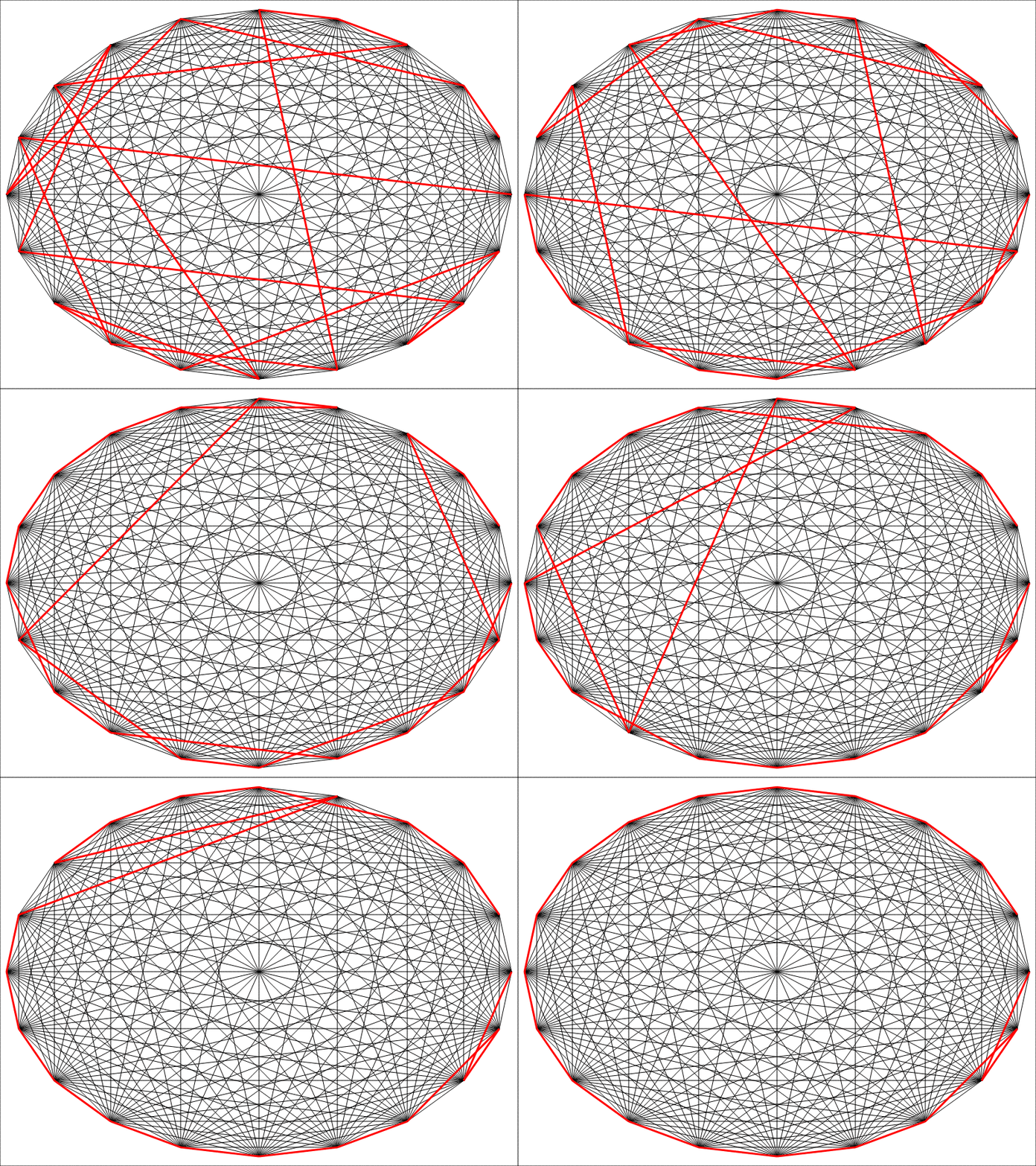
Ant Colony - Best Path - Animated.gif

Pheromones

  • Greater Usage => More Pheromones
  • Shorter Path Length => More Pheromones Remain
  • More Pheromones => Higher Probability of Usage
Pherimones 800x800.jpg

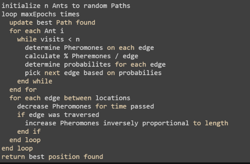
Ant Colony Optimization

Ant Colony Optimization Psudocode.png
 

Ant Colony Optimization

  • Neighborhood Search
    • Start with random paths
    • Explore neighboring paths based on probability
    • More pheromone = Higher probability of use
    • Can get stuck in a local minima
  • Tweaks
    • Number of ants
    • Pheromones to dispense
    • Pheromone dissipation rate
  • Features
    • Less sensitive to scale
    • Optimality not guaranteed
Ant Colony 800x800.jpg

Bee Colony Optimization

Bee Colony - Best Path - Animated.gif

Types of Bees

Active Workers
Forage on their known path and on a neighboring path

Scouts
Forage on a random path

Inactive Workers
Wait for information from other bees
Bee Colony 800x800.jpg

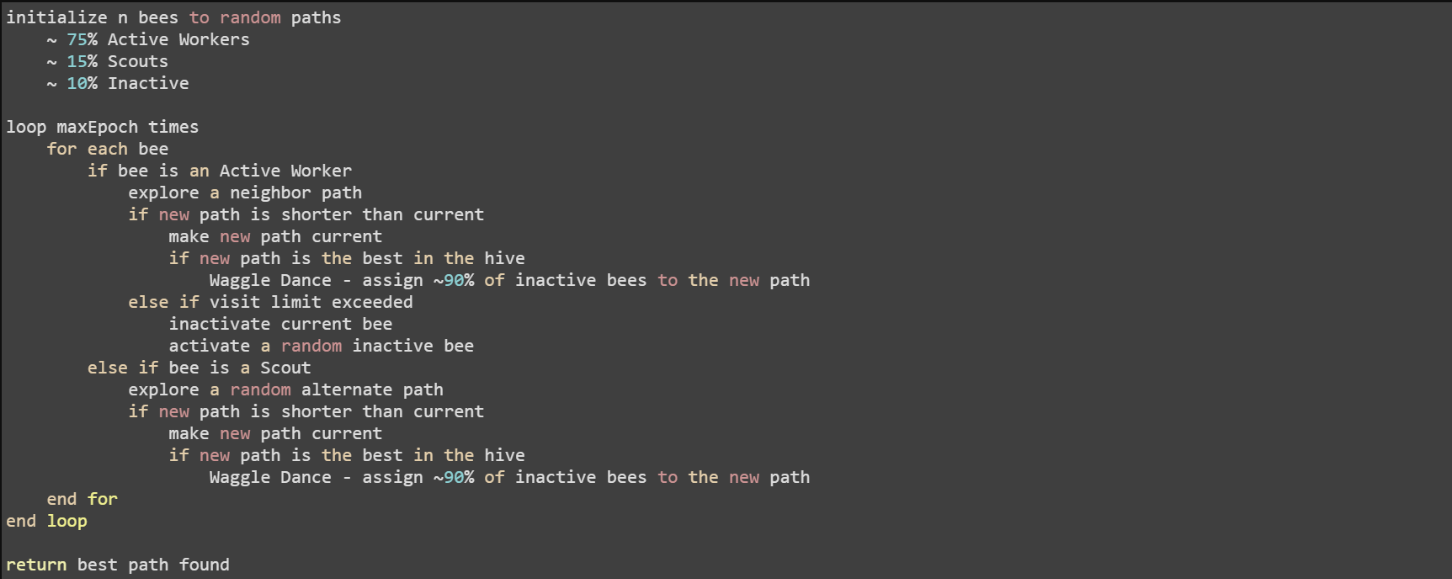
Bee Colony Optimization

Bee Colony Optimization Psudocode.png
 

Bee Colony Optimization

  • Multiple Search types
    • Active Workers perform neighborhood search
    • Scouts perform random search
    • Best known path propogates
  • Tweaks
    • Number of each type of bee
    • Probability of persuasion
    • Visit limit
  • Features
    • Less Sensitive to Scale
    • Optimality not guaranteed
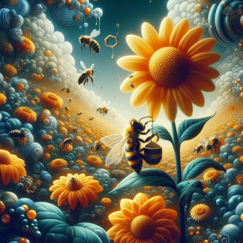
Bee Colony Optimization 800x800.jpg

Reducing Costs


Firefly Optimization

initialize n fireflies to random positions
loop maxEpochs times
  for each firefly i
    for each firefly j
      if intensity(i) < intensity(j)
        compute attractiveness
        move firefly(i) toward firefly(j)
        update firefly(i) intensity
      end for
    end for
  sort fireflies
end loop
return best position found
 

Firefly Optimization

  • Neighborhood Search
    • Search the area toward best known solution
    • Closer and Brighter: More Attractive
      • Similar to gravity
  • Tweaks
    • Number of fireflies
    • Range of possible values
    • How fast fireflies move
  • Features
    • Works better for linear problems
    • Optimality not guaranteed
    • Can suffer from sparseness problems
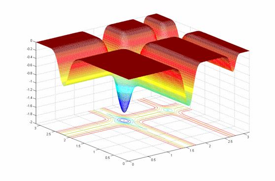
MichalewiczFunction.jpg


Amoeba Optimization

Amoeba Optimization - Solutions.png

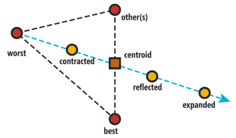
Amoeba Optimization

initialize the amoeba with n (size) locations
loop maxEpochs times
    calculate new possible solutions
        contracted - midway between centroid and worst
        reflected - contracted point reflected across centroid
        expanded - beyond reflected point by a constant factor
    if any solution is better than the current
        replace worst value with best value from new solution
    else
        shrink (multiple contract) all lesser nodes toward the best
    increment epoch count
end loop
return best position found
 

Amoeba Optimization

  • Neighborhood Search
    • Start with random locations
    • Explore neighbors based on amoeba movement
    • Surround the solution, then contract to it
  • Tweaks
    • Size of the amoeba
      • > # of search dimensions
    • Number of executions
      • Handle local minima
  • Features
    • Optimality no guaranteed
    • Can suffer from sparseness problems
MichalewiczFunction.jpg

What Can We Do With This Stuff?

Gradient Descent

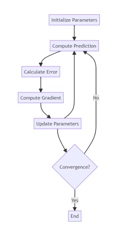
Optimization algorithm used to minimize the cost function of a model

  • Shifts the parameters in the opposite direction of the cost gradient

    • The 1st derivative of the cost function

    • Represents the slope of that function

  • Hyperparameters include:

    • Number of iterations

    • Learning rate

    • Convergence criteria

  • Stochastic Gradient Descent

    • Updates parameters using a subset of data each cycle
AI Models - Gradient Descent - 400x800.png

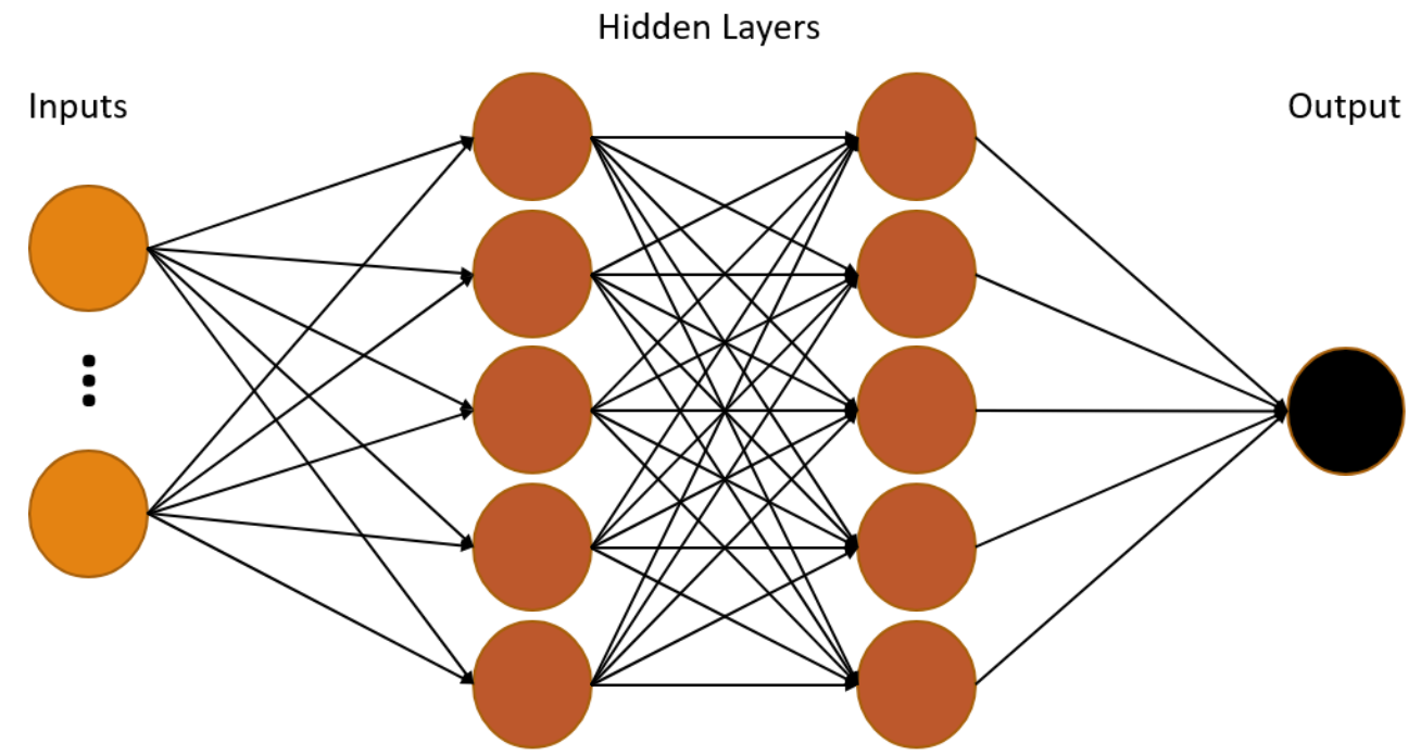
Deep Neural Networks

DNN.png


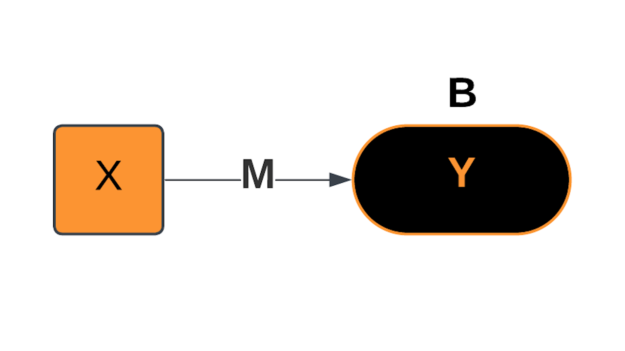
Linear Model

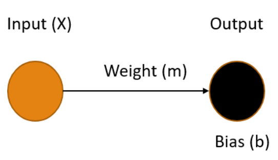
Component Details
Input Variable X
Output Variable Y
Weight Parameter M
Bias Parameter B
Linear Equation Y=mX+b
AI Models - Single Input Linear - 1280x720.png

ML's Linear Linchpin

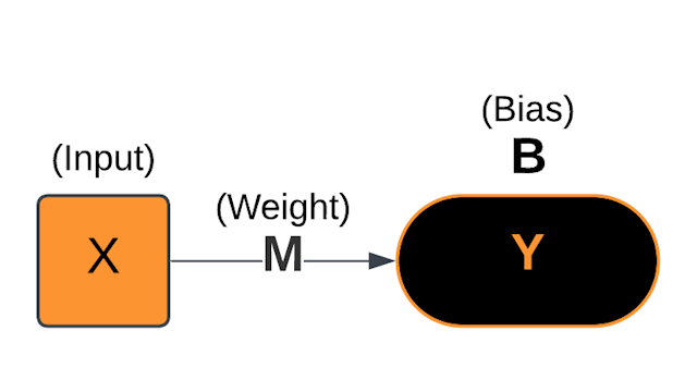
Y = mX + B

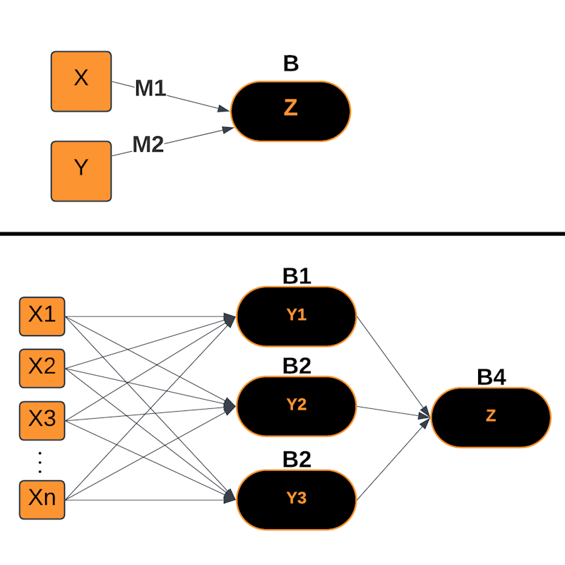
  • Every neuron gets its value from a linear transformation

  • Multiple inputs result in a sum of the linear transformations

    • The sum of a linear transformation is linear
  • Only linearly-separable functions can be modeled without a non-linear activation

AI Models - Annotated Single Input Linear - 640x360.png

Model Parameters

  • Parameters: Internal values learned during training

    • Define the relationship between input and output

    • Adjusted to minimize prediction error

  • In Linear Regression: Y = mX + b

    • m: Slope (Weight) - The influence of X on Y

    • b: Intercept (Bias) - Shifts the output vertically

  • In more complex models:

    • Counts include weights/biases across layers

    • Can capture non-linear relationships

    • Parameter counts are a proxy for complexity

    • GPT-4 uses roughly 1.8 trillion parameters

Model Parameters.png

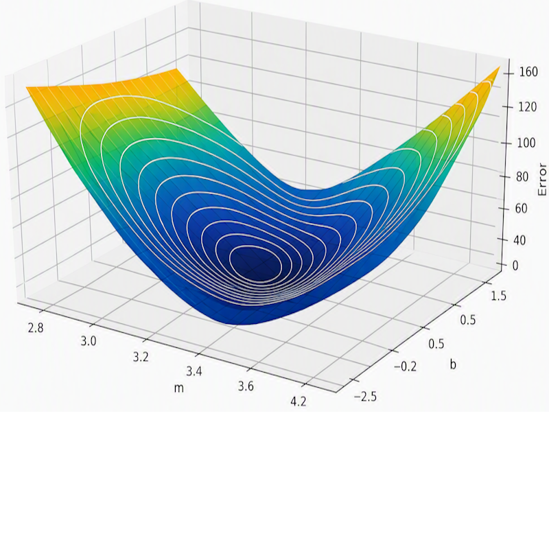
Error Function

  • X-Axis: The value of the weight (m)
  • Y-Axis: The value of the bias (b)
  • Z-Axis: The size of the error

The weight (m) often has a greater effect on the error than the bias (b)

Linear Regression - Error Function Plot - Smaller.png

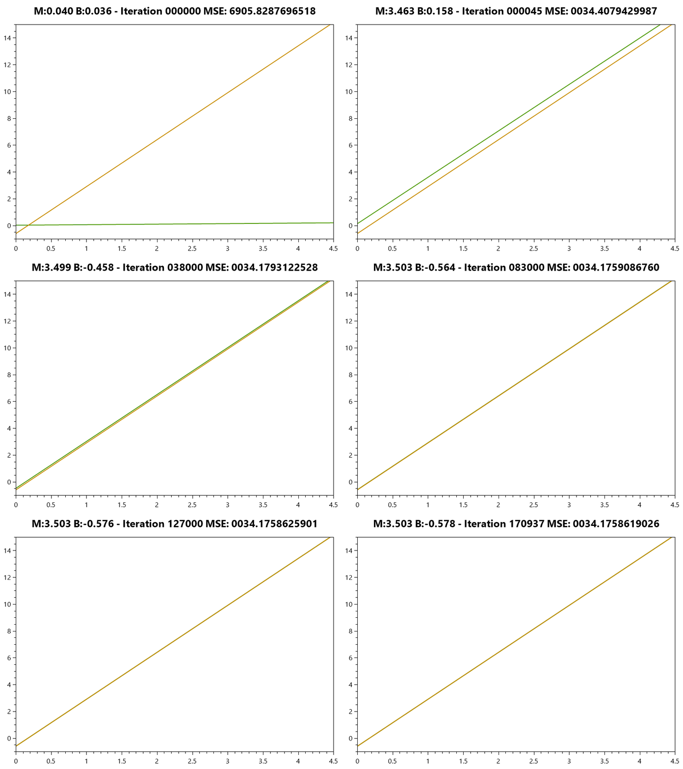
Training the Model

  • Objective: Minimize the error
    • Error: The difference between the predicted value and the actual value
    • MSE: Mean Squared Error - Avg of the squared differences between predicted and actual
  • Means: Gradient Descent Optimization
    • Nearly any Optimization algorithm can be used
    • Gradient Descent is the most common/suited
training_animation.gif

Linear Regression Demos

Linear Model Demos 800x800.jpg

Mathematics

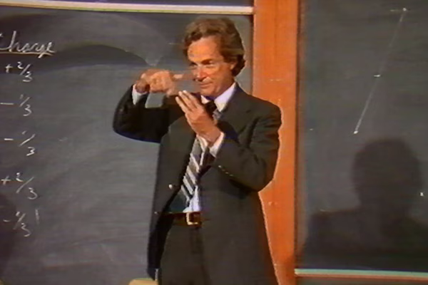
Feynman - QED - 600x400.png

...we've invented a fantastic array of tricks and gimmicks for putting together the numbers, without actually doing it. We don't actually [apply \(Y = mX + b\) for every neuron] We do it by the tricks of mathematics, and that's all. So, we're not going to worry about that. You don't have to know about [Linear Algebra]. All you have to know is what it is, tricky ways of doing something which would be laborious otherwise.


With apologies to Professor Feynman, who was talking about the tricks of Calculus as applied to Physics, not the tricks of Linear Algebra as applied to Machine Learning.

Train & Test Cycle
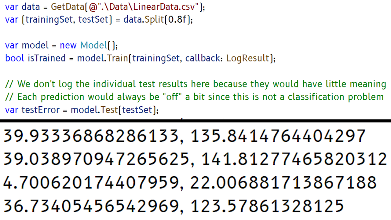
Train and Test Cycle.png


Railroad Times Model

AI Models - Single Input Linear - 1280x720.png

Linear Regression Model

Predict the unknown values in a linear equation​

  • Given X (time), predict Y (location)​
    • Y = mX + b​
  • Find the best values for m and b
    • Minimize total error
Regression Model.png

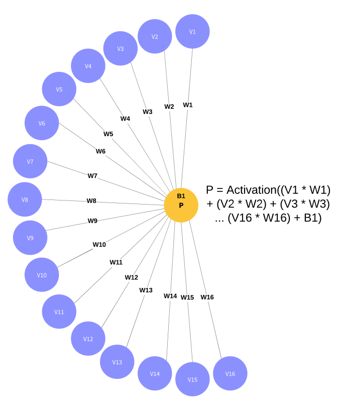
Voter Model

Voter Network Diagram - 673x800.png
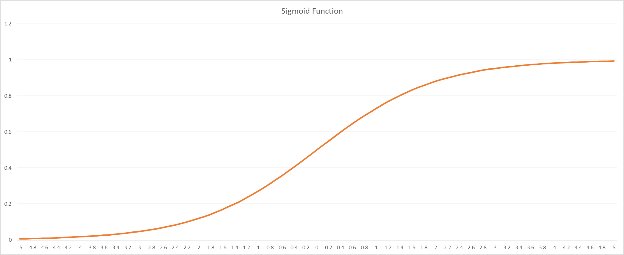
  Sigmoid Function.png
 

ML Demo

Using Amoeba Optimzation to Train an ML Model


More Bio-Inspired

  • Roach Infestation Optimization
  • Particle Swarm Optimization
  • Multi-Swarm (Birds) Optimization
  • Bacterial Foraging Optimization
More Algorithms 800x800.jpg

Solving Tractable Problems

  • Understand the Problem Deeply

    • Clarify inputs, outputs, constraints, and goals

    • Is optimality required? Can constraints be relaxed?

    • Identify if it can be broken into reusable parts?

  • Classify the Problem Type

    • Search? Optimization? Graph traversal? Dynamic programming candidate?

    • Are brute-force or exponential-time solutions feasible?

    • What tools do we have that can help? Can we buy vs build?

  • Implement and Test

    • Try a naive solution 1st

    • Use test cases to validate correctness and performance

    • Optimize as needed / Start over if necessary

Resources - Page 1

Amazing Algorithms - Short Workshop - QR.png

Resources - Page 2

Amazing Algorithms - Short Workshop - QR.png

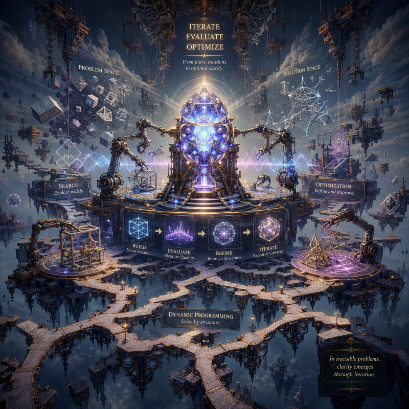
Solving Your Problems

Would you like to try to model a problem from one of your domains?